Microeconomics
Macroeconomics
SISTERetrics
SITES
Compleat World Copyright Website
World Cultural Intelligence Network
Dr. Harry Hillman Chartrand, PhD
Cultural Economist & Publisher
©
h.h.chartrand@compilerpress.ca
215 Lake Crescent
Saskatoon, Saskatchewan
Canada,
S7H 3A1
Launched 1998
|
Microeconomics 2.0 Demand
|
|
0.0 Introduction (MKM C20/463-82: 432-55; C21/460-483; 429-453) We begin construction of the Standard Model of Market Economics with Consumer Demand. This is where, historically, the model actually began. Its beginnings, however, still trouble many economists. In the world of Harry Potter "He Who Must Not Be Named " is Voldemort. In Economics it is Jeremy Bentham. In the late 18th and early 19th century Bentham reduced human behaviour to pleasure & pain: 'the sovereign rulers of the State'. He reduced them to an atom-like unit called a 'utile'. Using the utile, Bentham created a calculus of human happiness - felicitous calculus. In turn this calculus gave birth to the Administrative State (Part I, Part 2). And for purposes of Economics, most importantly, he assumed that how much money a consumer is willing to pay for a good or service is a measure of its 'utility'. For those interested in the historical and philosophical foundations of modern market economic thought please see: Observation #5: Jeremy Bentham. Those who dive into its murky waters will see why Economics is not accounting, business, commerce or mathematics but rather all of these and much more. We now begin constructing the model with consumer demand rooted in the concept of 'utility'. 1. Utility Function (MKM C20/449-50: 420-1; 449-450; & C21/472: 440; 469; 439) The atom-like unit, the utile, is a measure of the pleasure or pain enjoyed by a consumer in consuming a good or service. The utile exhibits distinct characteristics. First, and for Economics most important, the willingness of a person to pay a money price for a good or service measures how many utiles of happiness they expect to receive in exchange. This is reification – making concrete (money) something that is abstract (happiness). Furthermore, it is assumed that goods are infinitely divisible. Second, total utility is the satisfaction of consuming a total quantity of a good or service. Third, marginal utility is the additional utility yielded by consuming one more unit of that good or service. Fourth, diminishing marginal utility means that at some level of consumption an additional unit yields less satisfaction than the preceding unit, i.e. total utility increases but eventually at a decreasing rate. Furthermore, diminishing marginal utility eventually turns negative becoming pain not pleasure, too much of a good thing. Take the example of a good whose units in consumption generate the following number of utiles: 5, 4, 3, 2, 1, 0, -1, -2.... It is important to note that if, for example, a consumer gives up the third unit generating 3 utiles then the second unit is worth 4 utiles. What this means is the reverse of diminishing marginal utility each unit given up is worth more than the previous unit given up; Fifth, diminishing marginal utility means a person does not consume just one good. One does not live by bread alone. Assuming rationality, a person chooses that combination of two or more goods and services that maximizes total utility. This is calculatory rationality meaning every choice is a calculation of the number of utiles, a.k.a., happiness or pleasure. Furthermore, in theory, the consumer is assumed rational, i.e., one chooses between alternative commodity combinations to maximize utility assuming: a) perfect knowledge, that is, the consumer is aware of all alternative commodity combinations, their prices and resulting utility; b) competence, that is, a consumer is capable of evaluating the alternatives; and, c) taste of a consumer is transitive or consistent, that is, if a consumer likes A as much as B and B as much as C then one likes C as much as A. It is also assumed that the consumer is only able to order commodity combinations by level of utility, 1st, 2nd, 3rd etc. This is called ordinal measurement or rank ordering. Thus in consumption one does not specify the actual numeric level or utility known as cardinal measurement. Putting all these definitions and assumptions together we generate the consumption function as: (1) U = f (x, y) where: U is the utility derived from consuming combinations of x and y; f is the unique taste function of a consumer; U is continuous meaning there are infinite combinations yielding the same level of utility. Put another way, U is a dense set; a number assigned to commodity combinations such as U5 indicates only that it is preferable to combinations with a lower number, e.g., U4 and inferior to U6. In other words, we can rank order preferences but a U# has no cardinal meaning; and, U is defined for a specified timeframe that is long enough to allow substitution between commodity combinations but short enough to insure constancy of taste ii - Indifference Curves (MKM C20/465-70: 435-39; C21/463-468; 434-437) For any level of utility say U1 = f (x, y) there is a locus of commodity combinations which graphically form an indifference curve, first conceived in Edgeworth's Mathematical Psychics. All combinations on that curve have the same level of utility meaning the consumer is ‘indifferent’ to any point on the curve. The indifference curve is also called a preference or utility curve.
Usually an indifference
curve is ‘convex’ in shape reflecting that an increase in x can only
be obtained by a reduction in y, and vice versa
(B&P
7th Ed. Fig. 9.3;
MKM Fig. 21.2).
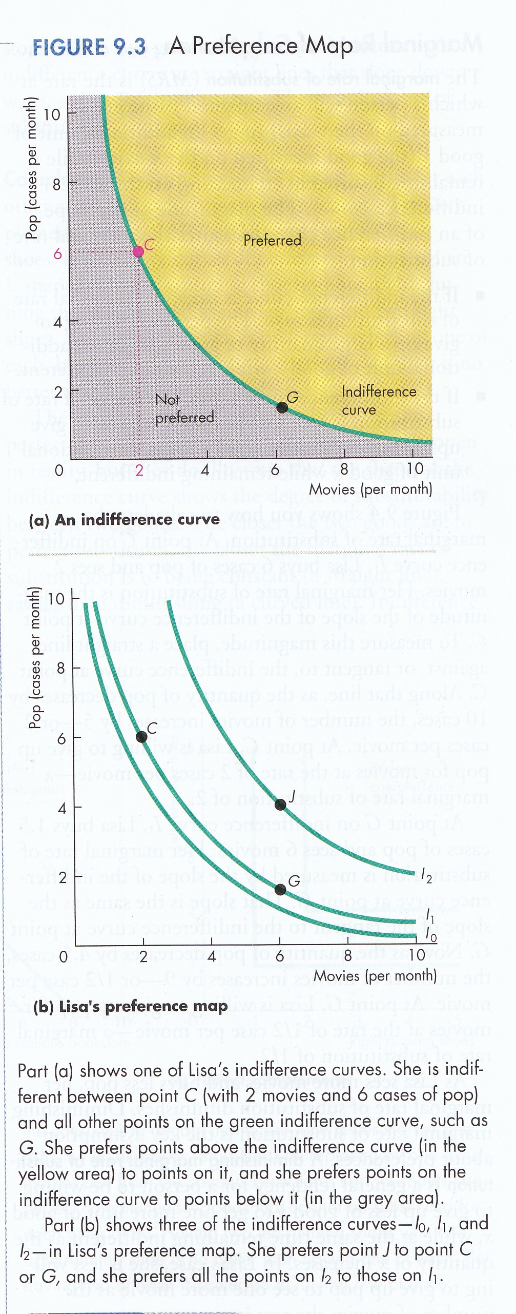
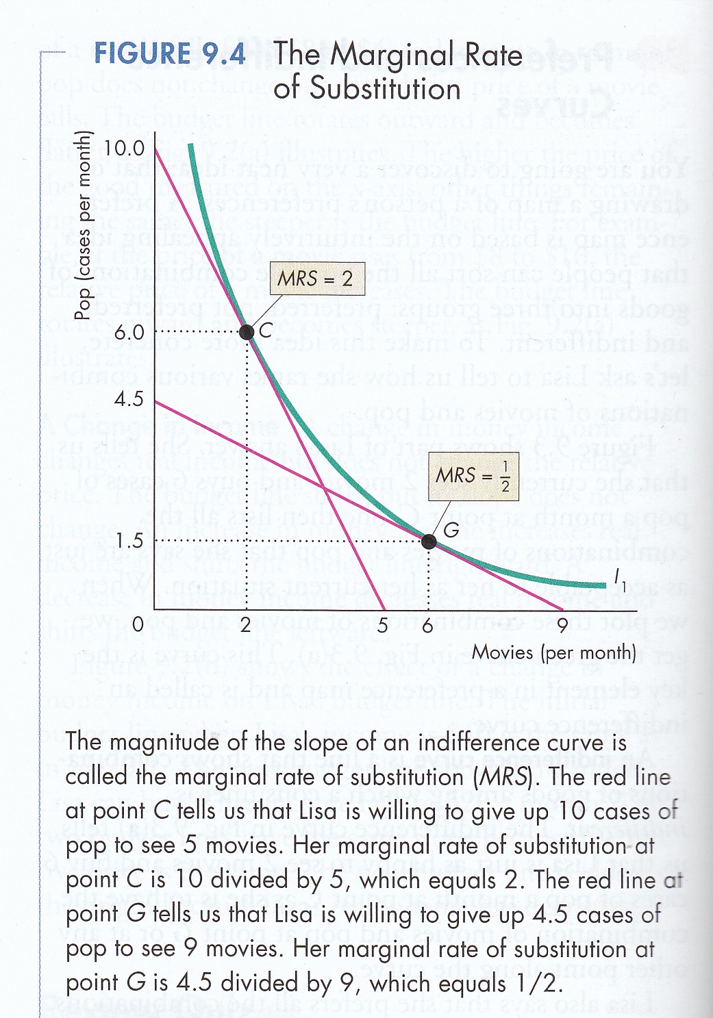
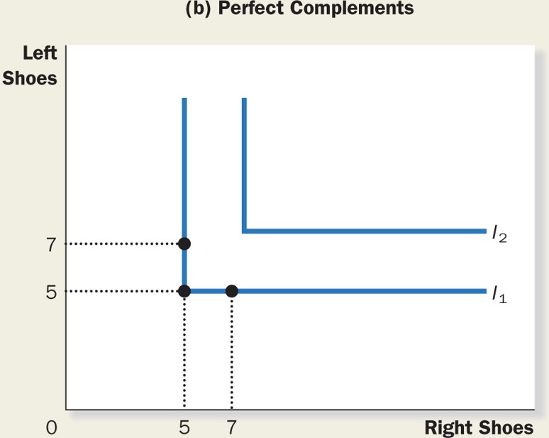
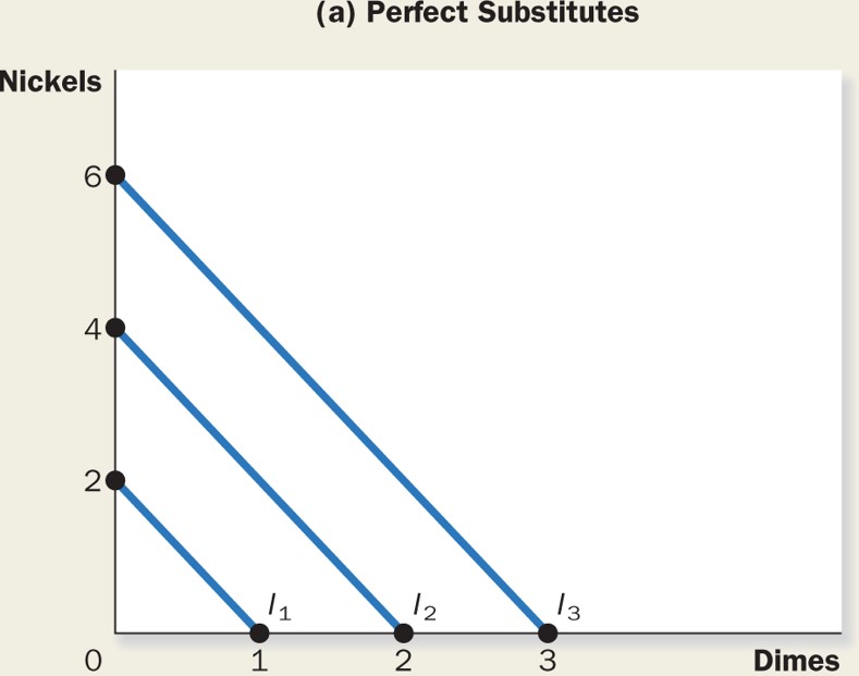
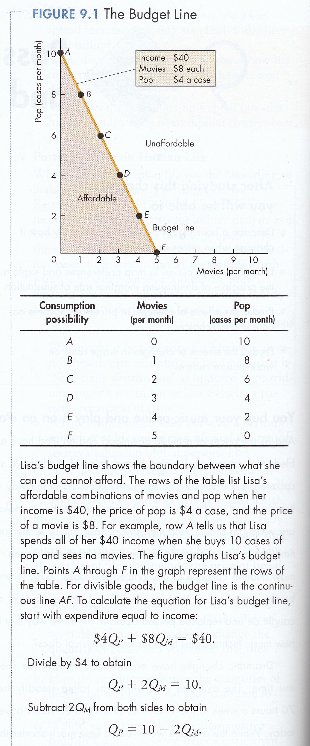
(2) MRS = MUx/MUy where: MRS = marginal rate of substitution MUy = marginal utility of y MUx = marginal utility of x (P&B 7th Ed Fig. 9.4; MKM Fig. 21.2; Fig. 21.3). As noted above ‘f’ in the equation U = f (x, y) is the taste function which is different for each consumer. Thus each consumer will have a uniquely shaped indifference curve and different MRS. When we plot all possible levels of U we get a set of curves forming a consumer’s indifference map. The transitivity assumption ensures the curves do not intersect but rather rise higher and higher. 2. Budget Constraint (MKM C20/464-65: 433-35; C21/461-463; 430-433) Before considering the Budget Constraint it is appropriate to consider the nature of goods & services purchased by a consumer and how they are able to pay their prices. Commodities are called ‘goods’ because they satisfy human want, needs and desires. i - Goods (MKM C20470 & 473; 437-438, 442; C21/465-467,469-470; 436-437, 440) Goods can be classified in different ways. First, there are complementary and substitute goods. Complementary goods are ones that are consumed together, e.g., hamburgers and French fries or IPods and IPod docking stations (MKM Fig. 21.5b; 21.6). Substitute goods are alternatives to one another, e.g., a bicycle is a substitute for a car in transportation. There are near and distant substitutes for most goods, e.g., a car or a truck are near substitutes while a car and a bicycle is a distant substitute (MKM Fig. 21.5a; 21.6). Second, there are normal and inferior goods. A normal good is one the consumption of which increases as income increases. An inferior good is one the consumption of which decreases as income increases. An example of an inferior good is cheap wine. As one’s income increases consumption of cheap wine tends to decline. Third, there are conspicuous consumption or Veblen goods (named after economist Thorstein Veblen) and normal consumption goods. Veblen goods are rare and their consumption goes up as price goes up in distinction from normal goods whose consumption goes down as price goes up. Conspicuous consumption goods are bought to demonstrate to others that one can afford such luxuries. ii - Prices To buy a good a consumer must pay its price. Further to Bentham’s assumption, the money price one is willing to pay for a good or service equals the satisfaction or utility one believes can be extracted from that good. iii - Income/Work To pay a price, however, one must have income. Income is earned through work which in the standard model is disutility, i.e., pain. One does not work for enjoyment (if one does one earns ‘psychic’ income) but rather for the monetary income used to buy goods and thereby derived satisfaction. iv - Constrained Maximization (MKM C21/470-472: 439-41; 467-468; 437-438) While a consumer wants to rise as high up the indifference map as possible, one is constrained by income (I) and the price of x and y. Thus for a given level of income and prices a budget line or constraint can be drawn. This constraint shows all combinations that can be purchased that exhaust income, i.e., (3) I = PxX + PyY where: I = income P = prices
X & Y =
quantity of goods
(P&B
7th Ed Fig. 9.1;
MKM Fig. 21.6; 21.7). One cannot consume above the constraint and, in this model, it is irrational to consume below (keeping cash on hand) because utility is derived only from consuming goods & services. The maximum amount of x or y one can afford (with a given income and prices) is shown by the intercepts of the budget line and respective axes, i.e., I/Px and I/Py (4) Price Ratio = Px/Py The slope of the Budget Constraint is ∆Y/∆X. To get the price ratio, however, an example will serve. Let us assume I = $10, Px = $2 and Py =$5. The maximum X a consumer can buy is 5 units; the maximum Y is 2 units. The slope of the Budget Constraint is ∆Y = (2-0) and ∆X = (5-0) or 2/5. Notice that this is equivalent to Px/Py = 2/5. Given the slope of the budget constraint is downward it is negative slope and the price ratio is expressed as (Px/Py). If income varies while prices remain fixed then a new higher budget line becomes available to the consumer parallel to the original. In other words higher income relaxes the constraint on one’s happiness. If, on the other hand, the price of X (or Y) decreases the slope of the budget line and therefore the price ratio changes. For example if Px goes down then the intercept which measures the maximum amount of X a consumer can afford increases even if income remains constant.
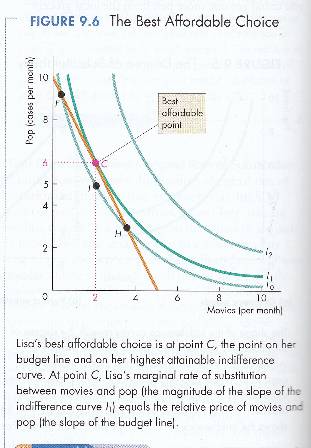
3. Equilibrium (MKM C20/470-2: 439-41; C21/467-468; 437-438) The combination of x and y that maximizes a consumer’s utility is the one on the budget line tangent or just touching the highest attainable indifference curve . This is the ‘best affordable point’ (P&B 7th Ed Fig. 9.6; MKM Fig. 21.6; 21.7) and satisfies the following conditions: (5) MRS = MUx/MUy = (Px/Py) that is the slope of the indifference curve or Marginal Rate of Substitution equals the slope of the Budget Line or the price ratio (Px/Py) and at this point the ‘rationale’ consumer equates the MU per dollar of each commodity consumed or (6) MUx/Px = MUy/Py where dollar-for dollar the additional utility from an additional unit of x is equal dollar-for-dollar to the additional satisfaction from one more unit of y. Consumers will remain at this point, i.e., be in equilibrium, as long as taste, income and prices remain fixed. This is the initial equilibrium. It is a condition which once achieved continues indefinitely unless one of the variables is altered. For our purposes there are two types: a) stable equilibrium: which refers to a condition which once achieved continues indefinitely unless there is a change in some underlying conditions. Changes in economic conditions will be followed by reestablishment of the original equilibrium. Example: a ball resting at the bottom of a cup; shake it and the ball moves; stop shaking and it returns to the bottom of the cup; and, b) unstable equilibrium: which refers to a condition which once achieved will continue indefinitely unless one of the variables changes but the system will not return to the original equilibrium. Example: a ball resting on the top of an overturned cup - shake it and the ball falls off never to return to the same place. (1) U = f (x, y) Utility Function (2) MRS = MUx/MUy Marginal Rate of Substitution (3) I = PxX + PyY Budget Constraint (4) Px/Py Price Ratio (5) MRS = MUx/MUy = Px/Py Consumer Equilibrium (6) MUx/Px = MUy/Py Equilibrium Condition
We will now change assumptions one by one and see what happens to equilibrium.
|
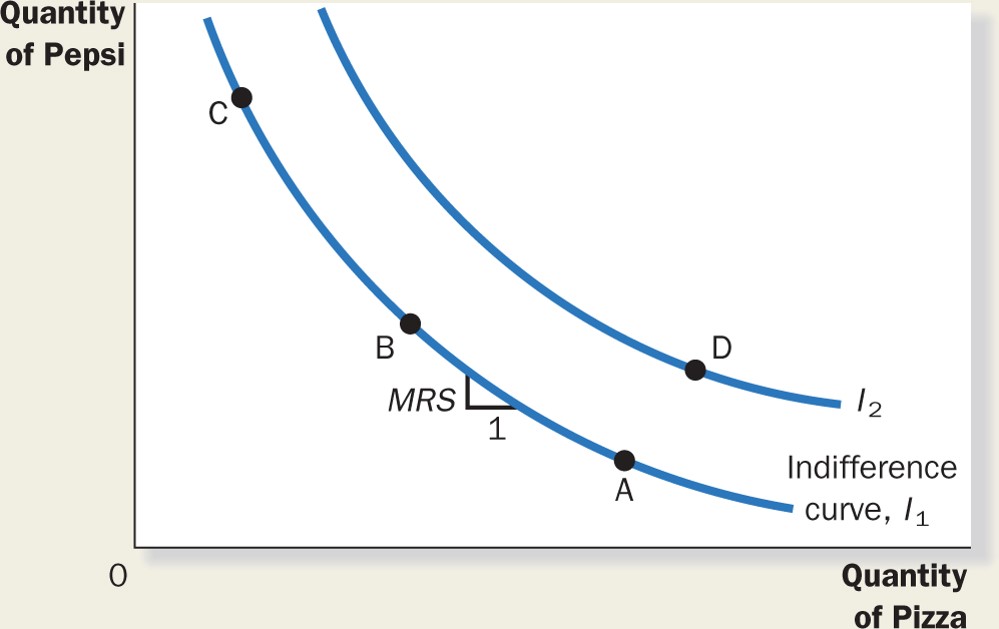 The amount of y that must be given up to get more x while
maintaining the same level of utility is the slope (rise over run)
of the curve at that point. It is called the marginal rate
of substitution, i.e.,
The amount of y that must be given up to get more x while
maintaining the same level of utility is the slope (rise over run)
of the curve at that point. It is called the marginal rate
of substitution, i.e., 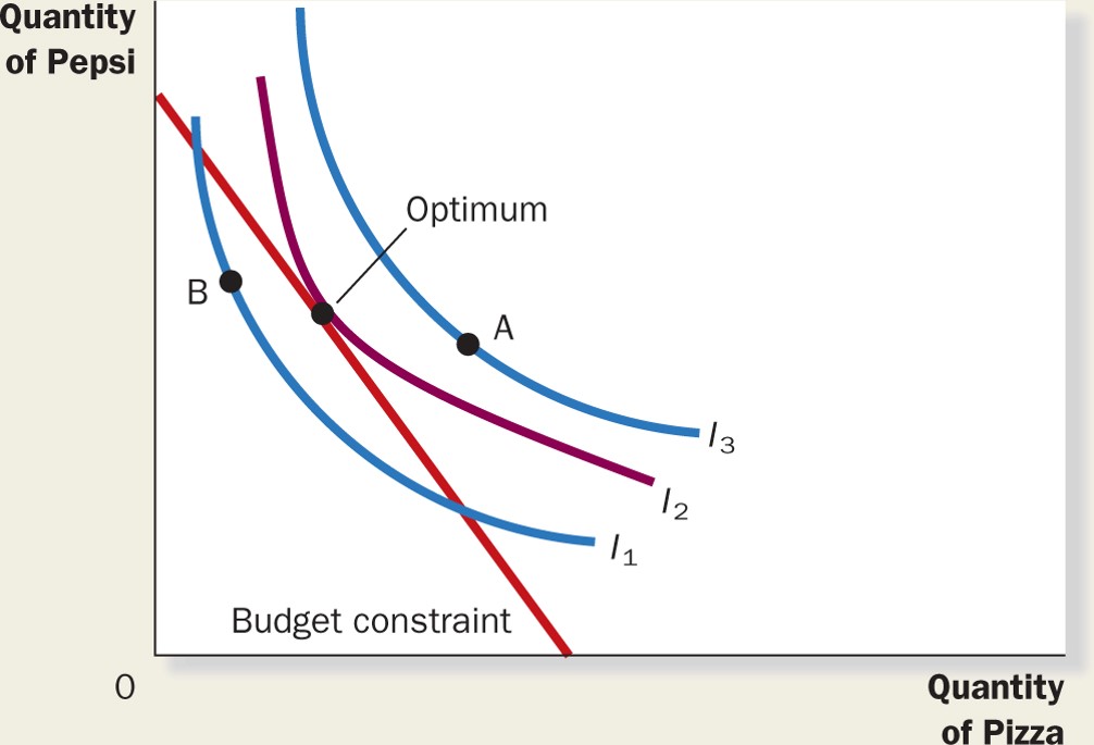