Microeconomics

2.0 Demand (cont'd)

1.  Initial Conditions (MKM CC21/460-483; 429-453)

   Maximum utility is found where the budget line is tangent to the highest attainable  indifference curve - that is, where the negative slope of the indifference curve (or marginal rate of substitution of x for y) is equal to the slope of the budget line, that is, the marginal rate of substitution equals the price ratio and here MU_x/P_x = MU_y/P_y.

2. Manipulations

  From the basic analytic mechanism of the indifference curve and budget line a range of additional information can be deduced including:

i - Income-Consumption & Engel Curves (MKM C21/472-3: 470; 439)

An increase in income shifts the intercepts of the budget line but leaves its slope constant - assuming constant prices.  The locus of tangents of budget lines with indifference curves forms the income-consumption curve (R&L 13th Ed Fig 6A-5), i.e., the set of commodity combinations (X, Y) consumed as income increases - assuming constant prices and taste.

From the income-consumption curve we can derive the amount of x purchased at different levels of income.  This forms the Engel Curve (M&Y Fig. 4.2) which, in effect, is the income demand curve for a good or service.  The shape of the curve depends on the type of commodity.  A normal good will have a positively sloped Engel Curve reflecting the fact that as income rises, consumption rises.  An inferior good will have a negatively sloped Engel Curve reflecting that as income increases consumption decreases.  An example is Kraft Dinner.  For a poor student it is a cheap source of pasta and cheese but when the student becomes a well-paid junior executive of a Fortune 500 company it is no longer preferred.

In business it is critical to know if one’s product is a normal or inferior good.  If consumer income rises then sales of a normal good will increase.  In a recession, however, with falling consumer income sales of a normal good decrease while sales of an inferior good increase.

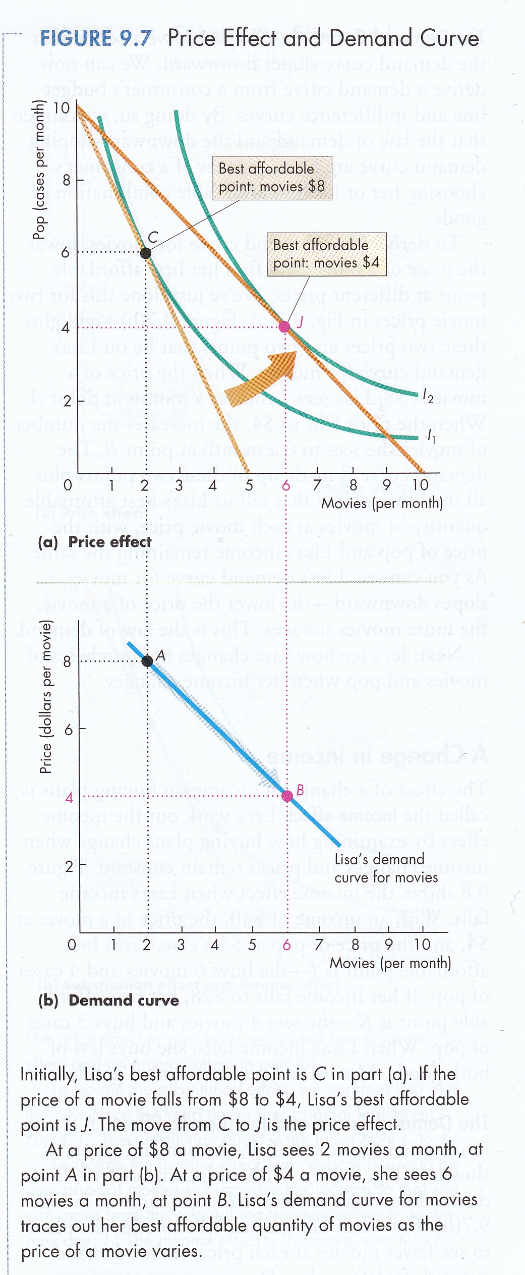
ii - Price-Consumption & Demand Curves (MKM C21/473-4; 477-8; 471; 440-441)

If the price of one commodity (X) changes a new set of combinations (X, Y) is created between the changing tangents of the budget line and indifference curves forming the price-consumption curve for the commodity.  The price-consumption curve shows how much of both commodities are purchased if its price changes - assuming constant income and prices for all other goods.

The demand curve for a commodity (X) can be derived from the price-consumption curve showing how much of that commodity is purchased at different prices - assuming constant income and constant prices for the other good (Y).  The shape of the demand curve (X) depends on taste, income and the type of commodity - assuming constant prices for the other good (Y) (P&B 7th Ed Fig. 9.7; R&L 13th Ed Fig. 6A-7, MKM Fig. 21.9).  The Law of Demand generally holds: the higher the price, lower the demand; lower the price, higher the Demand.  Why?  The Law of Diminishing Marginal Utility.

iii - Substitution & Income Effects (MKM C21/474-7; 472-473; 441-433)

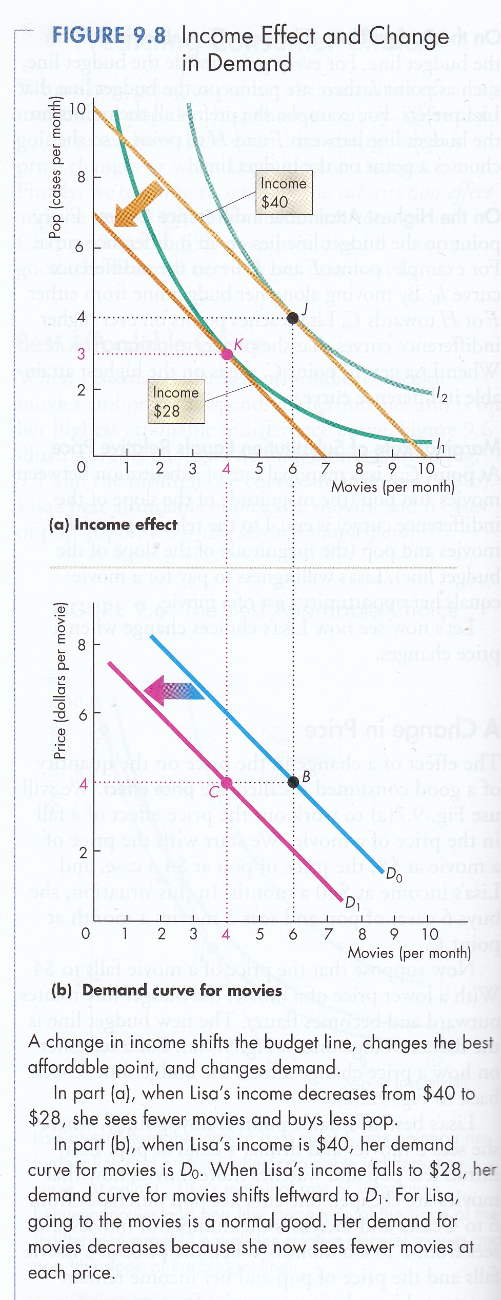
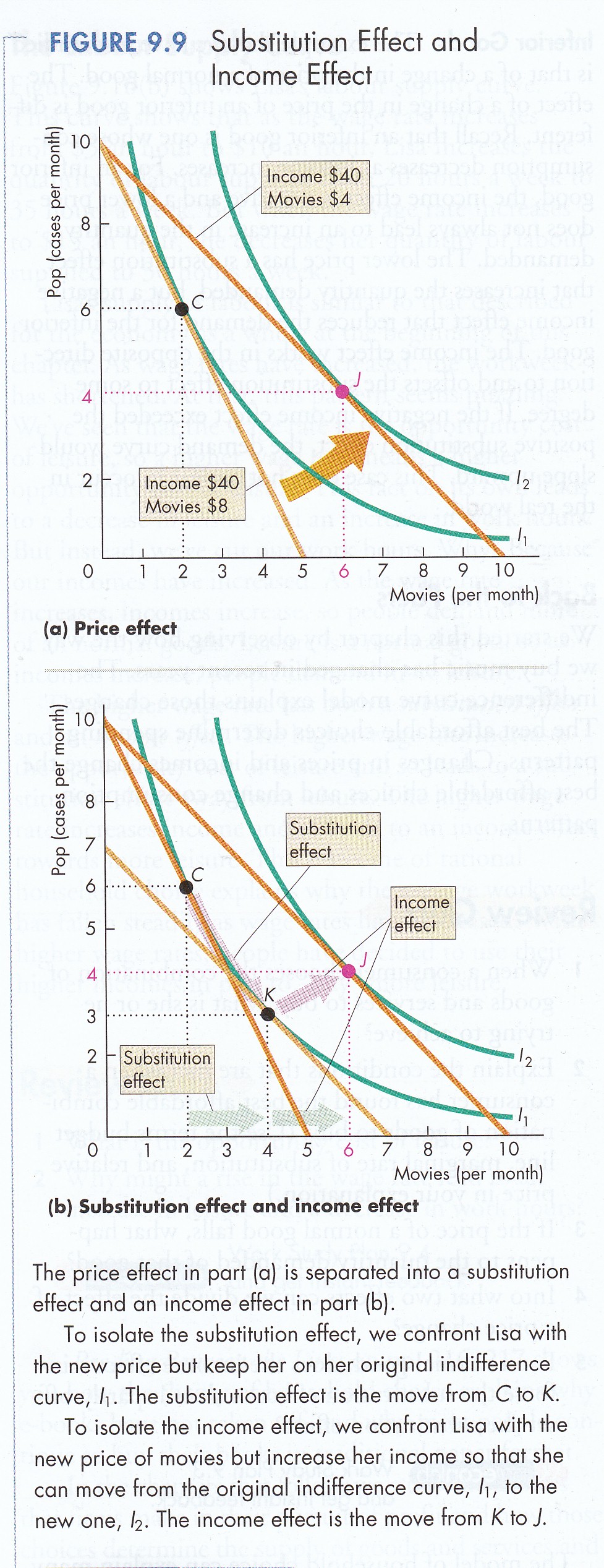
It is important to note that the change in price of one good or service (assuming income and prices of other goods remain fixed) has two effects.  For example, as the price of one good (X) declines it becomes cheaper relative to (Y). In equilibrium we have seen that consumers equates the marginal utility per dollar of each good, i.e., MUx/Px = MUy/Py.  If the price of (X) goes down while the price of (Y) remains constant then dollar for dollar the consumer can get more utility by substituting X for the now more expensive Y.  This is called the substitution effect.  This effect holds for both normal and inferior goods.

In addition, if the price of X goes down the consumer can now afford to buy the same amount but have income left over.  In effect income goes up allowing the purchase of more of both X and Y.  This is called the income effect. 

The substitution effect is always negative, that is if the price of a commodity (X) goes up, the quantity consumed goes down.  The income effect can be positive or negative.  For 'normal' goods, an increase in income results in an increase in consumption.  If the quantity decreases when income increases the commodity is an 'inferior' good.  In most cases, if the price of an inferior good decreases consumption will still increase if income rises. 

Taken together the substitution and income effects are called the price effect (P&B 7th Ed Fig. 9.9; R&L 13th Ed Fig 6A-5; M&Y 4.6, MKM Fig. 21.10).

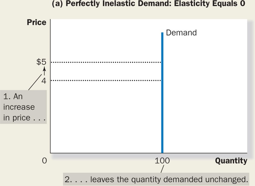
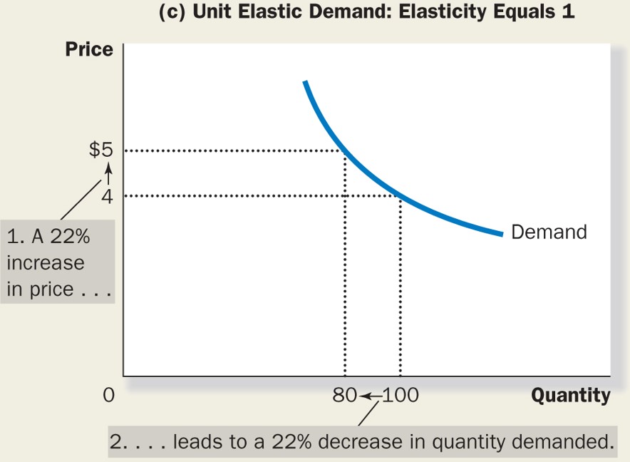
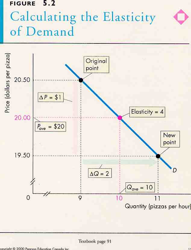
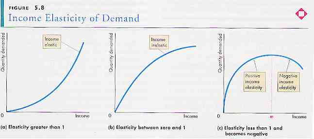
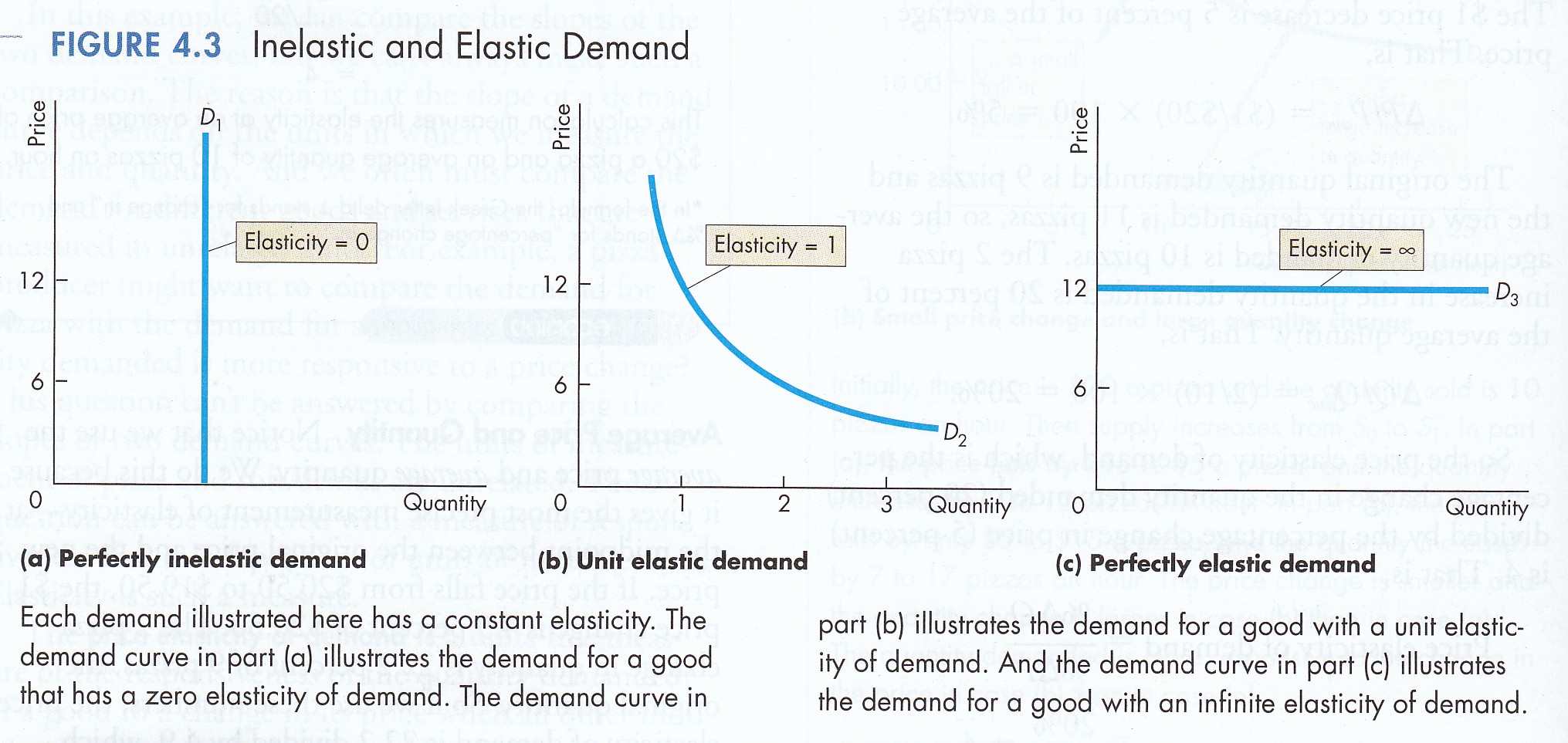
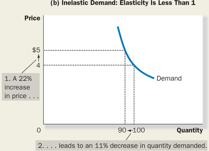
3. Elasticity (MKM C5/98-108; 97-117; 86-105)

Elasticity refers to the sensitivity of one variable to a one percentage change in another.  Economic theory recognizes three principal types:

i - income elasticity of demand  with prices constant refers to the percentage change in the quantity of a commodity demanded compared to a one percent change in income.  If income goes up 1% what happens to demand?  If it too goes up 1% there is unitary elasticity.  If demand goes up more than 1% there is elastic demand; if it goes up less than 1% then there is inelastic income demand for the good or service (P&B 4th Ed, Fig 5.8);

ii - price elasticity of demand refers to the percentage change in the quantity of a commodity demanded compared to a one percentage change in its price.  The amount demanded can increase:

a) more than proportionately, i.e. elasticity is greater than one - at the extreme a horizontal demand or supply curve is perfectly elastic - a small increase in price results in a large change in the quantity demanded or supplied;

b) proportionately, i.e. elasticity is equal to one (unitary elasticity); or,

c) less than proportionately. i.e. elasticity is less than one (inelastic) - at the extreme, a vertical demand or supply curve is perfectly inelastic - any change in price results in no change in the amount of the commodity demanded or supplied (P&B 4th Ed. Fig. 5.8; 7th Ed Fig 4.3; R&L 13th ED. Fig. 4-2 & 4-3, MKM Fig's 5.1 a, b, c & d);

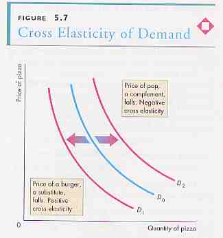
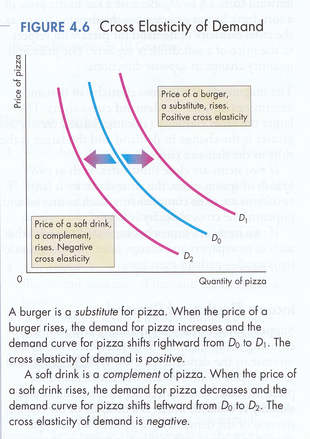
and,

iii - elasticity of substitution or cross-elasticity in the consumption of one commodity substituted for another by a consumer in response to a change in their relative prices (P&B 7th Ed Fig. 4.6).

In conclusion, consumption is the use of a product whereby utility is destroyed.  Put another way it is ‘negative production’.  Producers put utility into a good or service to satisfy human wants, needs and desires then consumers extract it.  Income is payment for work used to buy goods and services to obtain utility.  Work is the physical or intellectual effort made to earn income to purchase products and thereby obtain utility.  In and of itself, work is disutility or pain.  It is done only to earn income to buy goods & services and thereby derive utility.  Price is the dollar and cents cost of a product which is assumed to represent the utility a consumer can derive from it. 

Symbolic Summary of Demand

(1)  U = f (x, y)                                        Utility Function

(2)  MRS = MUx/MUy                            Marginal Rate of Substitution

(3)  I = PxX + PyY                                  Budget Constraint

(4)   Px/Py                                              Price Ratio

(5)   MRS = MUx/MUy = Px/Py              Consumer Equilibrium

(6)   MUx/Px = MUy/Py                          Equilibrium Condition