MBA 7003 1.2 Basic Conditions Supply

Supply refers to the willingness of producers to provide a given quantity of output at a given price. Such willingness reflects the production function of each firm inclusive of technology, the cost of inputs and the revenue received for its output. All things being equal ‘The Law of Supply’ is operative, i.e., the higher the price the greater the supply, the lower the price, lower the supply. There is therefore an upward sloping supply curve. Why? As we will see: the Law of Diminishing Marginal Product.

In Industrial Organization, the firm is located in four dimensions. First, buyers and sellers exchange of goods and services in markets – geographic, commodity-based and/or virtual, e.g., Ebay. Second, a firm or enterprise is any entity engaging in productive activity - with or without the expectation of profit. This includes profit, nonprofit and public enterprise as well as self-employed individuals. All enterprises have scarce resources and are accountable to shareholders and/or the public and the courts. A firm or enterprise is defined in terms of total assets and operations controlled by a single management empowered by a common ownership. Third, an industry is a group of sellers of close-substitutes to a common group of buyers, e.g. the automobile industry. Fourth, a sector is a group of related industries, e.g. the automobile, airline and railway industries form part of the transportation sector. Often ‘sector’ and ‘industry’ are used interchangeably, for example - the biotechnology industry or sector.

In the standard model of market economics, a.k.a., Microeconomics, a firm is a technical unit engaged in the production of one or a group of very closely related commodities. In theory, it is a single product firm with the entrepreneur as a surrogate for a decision-making hierarchy. It is the study mainly of external behavior and internal cost analysis, i.e. it not about business management. Furthermore, profit maximization is the only goal of the firm.

g = some function reflecting ‘know-how’ in combining factors to produce into outputs

The production function is time sensitive. However, the short- and long-run in economics is measured not in chronological time but in functional time, e.g., how long it takes to build a new plant. Thus the long-run in the restaurant industry is chronologically shorter than in the steel or nuclear industries but both are functionally the long-run in their respective industries. There are three types of time periods. To graph in two dimensional space only K and L are considered.

In the very short run, or what Marshall called ‘the market period’, output is fixed. All factors of production are fixed – labour, capital and natural resources. The very short-run supply curve is vertical and does not change with price. An example is the farmers’ market where produce is brought into the city from the farm for sale. No more produce is available. What is on hand is all that can be sold, no matter price.

In the short-run at least one factor of production is fixed, generally capital plant and equipment. More or less labour and natural resources can be employed and output increased or decreased.

With capital fixed and labour variable in the short run we can graph the production function as an 'S' shaped curve. Initially as labour is added its marginal product increases up to about 2.5 units in the graph (increasing MP_L) and then it begins to decrease from 2.5 up to 6.5 units (diminishing MP_L) becoming zero at the peak of the curve and then turns negative (negative MP_L). No profit maximizing firm will expand by hiring more labour if total output is decreased, i.e., beyond the peak of the production curve. There are, of course, some firms such as State owned companies in China that are not profit maximizers but rather employment maximizers.

Why does MP_Leventually decline and become negative. The simple answer is that capital is being spread thinner and thinner among more and more workers reducing their marginal product. In addition more and more workers means increased congestion and complexity. This is called the law of eventually diminishing product which has significant implications for the costs of a firm as output rises. It parallels the law of eventually diminishing utility in Consumer Theory, i.e., eventually the marginal utility of a good declines and becomes negative, too much of a good thing makes you sick. The marginal product of labour, i.e., the additional output generated by employing one more unit of labour is measured by the slope of the production function. The average product of labour, or the average output of all workers, is measured by the slope of a ray, i.e., straight line, from the origin where it intersects the production function. It should be noted that some rays will intersect the production function at two points. At each of these two points marginal product is the same. As will be seen this has significant implications for the shape of the marginal and variable costs curves of a firm, specifically their 'U' shape. As will be seen, if we know the cost of labour we can calculate the marginal cost of an additional unit of output and the average variable cost of any given level of output.

In the long-run all factors of production are variable – capital plant & equipment, labour and natural resources.

As noted previously modern microeconomic theory began with demand and the constrained maximization of utility by the consumer demonstrated using indifference curves and budget constraint. Initial attempts to explain production adopted the same basic mechanism with one important change: measurement of output is cardinal. That is we can, unlike utiles, count the exact number of units being produced. The firm thus wants to maximize output (Q):

The firm, however, faces a constraint: the cost of inputs or factors of production. In symbolic logic, this cost constraint is:

Assuming all factors are infinitely divisible then different levels of Q can be produced using different factor combinations. This generates an isoquant a curve representing a constant level of output all along its run (R&L 8A-1; M&Y 10th Fig. 8.2). The slope of the isoquant is the marginal rate of technical substitution (MRTS) of capital for labour maintaining the same Q. In symbolic logic it is

There are theoretically an infinite number of isoquants rising to higher and higher levels of output (R&L 8A-2). They are convex to the origin (opening away) due to the Law of Diminishing Marginal Product which states that as one factor is given up in favour of another eventually marginal product of the increasing factor will decrease.

While the firm wants to maximize Q it faces a cost constraint. For a given cost a maximum amount of capital or labour can be bought illustrated by the intercepts of the x- and y-axis. Its slope is the relative cost of the two factors or in symbolic logic is:

As with the budget constraint price ratio by convention the cost ratio is the inverse of the slope of the resulting cost constraint curve. The curve shows all combinations of K and L that can be bought for a specific cost (R&L 8A-3; M&Y 10th Fig. 8.2). Maximum Q for a specific cost is achieved where the cost constraint just touches or is tangent to the highest attainable isoquant. At that point, the slope of the cost constraint equals the slope or MRTS of the isoquant.

dollar-for dollar the marginal product of an additional unit of L is equal dollar-for-dollar to the marginal product of an additional unit of K

As with consumption and the Income Consumption Curve, if we relax the cost constraint while holding factor prices constant, a new cost constraint with the same slope (1/C_L/C_K) is created and a new equilibrium established. Repeating this process a locus of point is created all of which satisfy the equilibrium conditions (MP_K/C_K = MP_L/C_L) forming the expansion path for the firm (M&Y 10th Fig. 8.18).

This initial attempt to plot the supply curve of the firm was judged inadequate for the simple reason that factors of production especially capital are not infinitely divisible but rather ‘lumpy’ particularly in the short-run. A new approach was required that focused on the short-run behavior of the firm.

Before considering how to derive the supply curve of a firm it is appropriate to consider the inputs to the process. Factors of production or inputs are the ingredients used by a firm to produce a good or commodity. Traditionally there are three capital, labour and natural resources. Their meaning has, however, evolved over time. My summary of the evolution of the production function follows description of factors of production as Exhibit 1 (below).

The concept of capital has mutated and expanded through the history of capitalism. To the Mercantilists of the 17th century, capital was gold, silver, land and slaves. To the Physiocrats of pre-Revolutionary France, it was the surplus generated by agriculture. To the Classical School of the late 18th and early 19th centuries, it was the surplus resulting from specialized physical plant and equipment combined with the division and specialization of labour. To the Neo-Classical School of the late 19th and 20th centuries, it was financial capital. To Bohm-Baverk and the Austrian School, capital was historically embodied labour produced through ‘round-about’ means of production (Blaug 1968, 510-11). How to measure such embodied labour has never, however, been satisfactorily answered (Dooley 2002). Today, when economists speak of capital, they may refer to cultural, financial, human, legal, physical, social or other forms expressed as a stock existing at a given moment in time. For our purposes, however, capital is restricted to physical plant and equipment and its equivalent financial value.

Labour, unlike capital, has been subject to definitional reduction rather than expansion. It has been subject to capitalization rather than humanization as a factor of production. Thus education and training add to the stock of ‘human capital’, something ideologically alienated from labour and subject to managerial control as a corporate or national asset. Similarly, entrepreneurship and management have become detached from labour even though separation of ownership from control – public or private - makes the manager an employee or agent, not a principal or owner. In effect, labour becomes warm hot bodies applying muscle not brains doing what it is told. Effort is organized according to a division and specialization of labour (brawn) determined by a specialized class of employee called management (brains). In fact there are three forms of Labour - (i) Productive, (ii) Managerial & (iii) Entrepreneurial.

Productive workers are those on the shop floor actually producing goods & services. They are concerned with output. Their knowledge is technical and specialized to a given industry or firm. In effect they combine codified and tooled with personal knowledge (memory and reflex) generally learned on the job in the Anglosphere. Their knowledge involves making something or making something work. In this sense the competitiveness of a firm or nation “depends not only on sensible decisions about what to do, but on the availability of the skills that are required to do it” (Loasby 1998, 143).

Management, among other things, means “a governing body of an organization or business, regarded collectively; the group of employees which administers and controls a business or industry, as opposed to the labour force”. It also means “the group of people who run a theatre, concert hall, club, etc” (OED, management, n, 6). The role of management is to make available the means (inputs) so that production workers can perform their tasks and then to market and distribute the output. In many ways management is like a choreographer, music or theatre director. This sense of modern management is caught by Aldrich:

Thus the total operation is a performing art with blueprints for score or choreography, the difference being that in this technological case neither the co-ordinated performances (ballet) of the skilled workers nor the finished product is put on exhibit simply to be looked at, contemplated. It is a useful performing art. Its value is instrumental.” (Aldrich 1969, 381-382)

the fit of the organizational elements, rather than the elements themselves, that characterizes a firm. Just as the quality of an orchestra performance cannot be adequately measured by the average quality of the performances achieved by the individual instruments, but depends crucially on the way the instruments are played together, so the productive value of a firm - as opposed to a set of individual contracting relationships - emerges from the quality that has been achieved through mutually adjusting the various activities that are carried on. (Schlicht 1998, 208)

One crucial characteristic of the firm is custom including tacit understandings of entitlements and obligations between productive, managerial and entrepreneurial workers. This constitutes part of what is commonly called ‘the corporate culture’ for which, on a day-to-day.

With the notable exception of firms like Microsoft (Bill Gates) and Walmart (Sam Walton), most modern corporations do not follow an original founder/owner but rather a ‘hired gun’, or business entrepreneur. The word ‘entrepreneur’ comes from the French entre meaning ‘between’ and prendre meaning ‘to take’. The English ‘middleman’ retains this original sense. During the Middle Ages and Renaissance, European traders (especially from Venice and Genoa) ‘middled’, at high risk, between foreign suppliers, e.g. of silk and spices from the Turks, and final consumers in northern Europe. Today the term usually refers to someone who sees and seizes an economic opportunity or a market opening or gap. This may take the form of a new product or of servicing an existing market in a new way. In both cases a high degree of creativity and risk-taking is implicit. In this regard, the first English usage of ‘entrepreneur’ was in 1828 meaning “the director or manager of a public musical institution.” Today we would call this ‘an impresario’. In fact, it was not until 1852 that entrepreneur took its modern meaning of “one who undertakes an enterprise; one who owns and manages a business; a person who takes the risk of profit or loss (OED, entrepreneur, a, b).

Entrepreneurial knowledge is intuitive in seeing and taking advantage of invariants and affordances in a market that others do not see. It involves seeing and realizing a vision of future markets, products and opportunities. Ignorance is the opposite of knowledge, i.e., want of knowledge. The non-rational way of entrepreneurial vision was called ‘animal spirits’ by Keynes (Keynes 1936, 161). Like some ancient priest-king, the entrepreneur ‘knows’ the future and leads his people (investors, managers, workers and consumers) into it – right or wrong - to success or failure. In a manner of speaking, prophets today seek profits, not souls. Ideally, this highly valued form of pattern recognition works best as “informed intuition” (Jantsch 1975). All available information, knowledge and opinion is explicated but then an intuitive, inductive judgmental vision is conjured up. In a sense, the business entrepreneur or CEO has assumed the mantle of the Western Cult of the Genius joining the artist, inventor and scientist.

At first glance, natural resources have no relationship to knowledge. By definition, they exist as John Locke said in “the State that Nature hath provided” (quoted in Dooley 2002, 4). They are just part of the environment until the knowing mind recognizes them as useful. Thus oil lay in the ground virtually untapped until invention of the internal combustion engine. Just as we recognize a tool by its purpose (M. Polanyi 1962, 56), we similarly identify natural resources by the human ends we attribute to them. At a given point in time a naturally occurring substance is seen as nothing but an environmental feature. Take a pathway through the jungle one day and you see a large rock outcrop. The next day, with new knowledge, the same path leads not to an environmental feature but to a bauxite deposit that can be converted into aluminum. It has become a toolable natural resource. Yet it itself has not changed, one day to the next, rather new knowledge allows us to see it in a different light. This ‘changed way of seeing’ is captured by Loasby when he writes:

Menger begins by arguing that an object becomes a good only when someone discovers how to use it to satisfy some human need. Goods are endogenous, created by new connections between human need and physical or human resources; and their value is derived from the need which each of them serves and - crucially for this paper - from the knowledge that it can serve this need and also the knowledge of how it can be made to do so… The creation of goods, and of technology, rests on the creation of knowledge, and therefore on previous uncertainty - or indeed sheer ignorance.” (Loasby 2002, 6)

Today the most striking example of how new knowledge transforms environmental features into toolable natural resources is biotechnology. While advances in analysis and sequencing now allow researchers (and hence firms) to experiment with known genetic command codes to build new drugs, enzymes, pathways, proteins et al, the reality is that the raw material for biotechnology is life itself – everywhere and every when. Nature is much older and more experienced in designing command codes under a wide range of environmental conditions than emergent biotechnology. Accordingly Nature has become the object of search by the biotech industry for novel code. This search is called ‘bioprospecting’ and takes two forms: ethnobiology and ‘original research’ which is self-explanatory. For our purposes, however, we will restrict factors of production to capital and labour.

Exemplar Economy

Sector

Production Function

Accreting Factors of Production

Spain

16^th, 17^th to mid-18^th centuries

Primary

farming, fishing, forestry & mining

Y = f (K)

K = gold, silver, land & slave labour

England

late 18^th to mid-19^th centuries

Secondary

manufacturing

Y = f (K, L)

K = manufacturing plant & equipment

L = division & specialization of free labourers

U.S.A.

late 19^th to mid-20^th century

Tertiary Services

communication, energy, financial, transportation

Y = f (K, L, T)

K = private financial capital & limited liability corp.

L = organized labour

T = disembodied, endogenous

Japan

mid- to late 20^th century

Government

Y = f (K, L, T) ^G

K = public & private capitalization

L = automated labour

T = embodied, exogenous

G = government coordinates public & private sectors through macro- & micro-economic policies

Global

late 20^th & early

21^st centuries

Quaternary

Y = f (K, L, P, O, D) ^G

K = knowledge capital

L = knowledge workers

P = physical technology

O = organizational technology

D = design technology

G = national innovation system ensures rapid commercial exploitation of academic or pure research to grow GDP

Assuming that at least one factor of production is fixed (usually capital), the production curve for total output shows an initially rising section that peaks and then declines if additional variable inputs are added (R&L 7-1; M&Y 10th Fig. 7.1). No rational producer will go beyond the peak. Why does the curve peak and then turn down? Congestion. With fixed capital plant and equipment additional labour initially increases output but eventually an additional worker simply gets in the way of other workers and output actually declines.

As additional workers are added each contributes to output. If we take total output at each level of employment we can calculate both the average output per worker and the marginal or additional output contributed by one more worker (M&Y 10^th, Fig. 7.2). As can be seen, the addition of a worker initially increases the average output per worker but then the average declines as the marginal output per additional worker gradually declines following the Law of Diminishing Marginal Product: the marginal product of any input will eventually fall as the employment of that input increases - assuming other factors of production are held constant.

The average product of labour can be calculated as the slope of any line from the point of origin to the total product curve (M&Y 10th Fig. 7.4). Similarly, marginal product can be measured as the slope of the total product curve (M&Y 10th Fig. 7.5).

Economic choice involves how to satisfy infinite human wants, needs and desires with scarce resources. It requires a choice between alternatives, e.g., a pensioner choosing food or medicine. The choice of the best alternative means the next best alternative is not chosen. Put another way, the cost of choosing one possibility is the next best alternative foregone. This is called ‘opportunity cost’. All economic costs are opportunity costs even those not expressed by market prices.

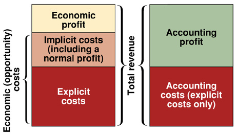
While for convenience one usually measures opportunity cost in dollars it actually involves real alternatives foregone. Thus for a firm, the opportunity cost of producing (OCP) a good (and therefore opportunity cost of employing factors of production) is the next best alternative action. There are two components to a firm’s OCP : explicit and implicit costs. Explicit costs are paid directly in money; implicit costs or opportunities foregone are not paid directly in money (even though measured that way). Explicit costs include direct payment for factors of production, e.g. in the case of labour, money cost or wages are generally equal to their OC. Implicit costs include the implicit cost of physical capital, inventories and the owner’s resources. (MBB 10th Ed. Fig. 7.1; P&B not displayed; R&L 13th Ed not displayed)

Assuming one factor of production is fixed (usually capital) then we are in the short-run and can identify three types of costs measured in three different ways.

In the short-run a firm can produce different levels of output but only by varying variable inputs. Accordingly the firm has three distinct types of costs:

i - fixed costs associated with the fixed factor of production - usually K but in the knowledge industries often L or 'the talent'. Fixed costs must be paid no matter the level of output, i.e. even if the firm shuts down fixed costs still have to be paid;

ii - variable costs associated with variable factors of production - usually L. Variable costs rise and fall according to how much of the variable factors are employed. The higher the level of production, all things being equal, the higher the variable costs; and,

iii - total costs that include all fixed and variable costs or TC = TFC + TVC (R&L 7-2; M&Y 10th Fig. 8.6).

In turn, for each type of cost at every level of production, average costs can be calculated:

i - Average Fixed Cost (AFC) = fixed cost per unit output (M&Y 10th Fig. 8.7). AFC will decline as output increases as the fixed cost is spread over a larger and larger level of output;

ii - Average Variable Cost (AVC) = variable cost per unit output (M&Y 10th Fig. 8.8). The distance between the AVC curve and the TC curve will tend to narrow as output increases because AFC declines as output increases; and,

iii - Average Total Cost (ATC) = fixed (AFC) + variable (AVC) cost per unit output (M&Y 10th Fig. 8.9).

In turn, for each level of production, marginal cost can be calculated from the additional cost associated with one additional unit of output (M&Y 10th Fig. 8.10). Average total and marginal cost can also be calculated from the total cost curve. Average total cost can be derived from the slope of a straight line or 'ray' drawn from the origin to any point on the total cost curve (M&Y 10th Fig. 8.123). Marginal cost can be derived from the changing slope of the total cost curve itself (M&Y 10th Fig. 8.13).

Marginal cost (MC) will initially decline as output increases but eventually, assuming at least one fixed factor of production, the Law of Diminishing Returns sets in and marginal cost begins to rise. The MC curve will cut the average cost curve (AC) at its lowest point. Thus as long as MC < AC then AC falls; when MC = AC then AC will be at its minimum; when MC > AC then AC will increase (R&L 7-2; M&Y10th Fig. 8.14).

Using the one fixed factor cost function, the long-run cost or expansion path of a firm is considered to be the sequence of short-run (SR) scenarios for varying scale of plant and equipment (M&Y 10th Fig. 8.15). In each SR scenario the scale of plant and equipment increases but during that period plant and equipment are consider to be fixed. The result is a set of average cost curve for each scale of production. An envelop curve can then be drawn representing the long-run (LR) minimum average cost at each level of output (M&Y 10th Fig. 8.16). The question remains as to when this series of SR scenarios becomes the LR.

The question remains: How much output will a firm be willing to supply given its cost constraints? Put another way: What is the firm's supply curve? This depends on how much the firm can get for its output, i.e. the price or revenue it receives per unit (R&L 9-4; M&Y 10th Fig. 9.3).

If a firm cannot earn at least enough to cover all of its variable costs then in the short run it will shut down. This occurs at point B where marginal cost is equal to minimum average variable cost. This is called the 'shut down point'. If a firm earns a price higher than B it can cover all of its variable costs and some of its fixed costs and it will stay in business. Put another way, the firm will maximize profits by minimizing losses.

In the long run, however, a firm must cover all costs - fixed and variable - or it will go out of business. This occurs at point D where marginal cost is equal to minimum average total cost. This is called the break-even point. At this point all factors of production - including entrepreneurship - are fully paid their opportunity cost. If the firm receives a price higher than the break-even point then it will earn economic or excess profits. Thus the supply curve of a firm is the marginal cost curve above minimum AVC (shut down point) in the short-run and above minimum ATC (break-even point) in the long-run.

It is important to appreciate that the price or revenue a firm receives applies to each and every unit of output it sells. Accordingly it will produce to the point at which the cost of the next unit of output (MC) equals the price or marginal revenue (MR) it receives for that last unit. In effect, a firm earns a profit on each previous unit (if the price or revenue is greater than minimum AVC or minimum ATC in the short- and long-run, respectively). A firm thus maximizes profits (or minimizing losses) by producing at the point where price or marginal revenue equals marginal cost of the last unit of output.

From the resulting cost function we can determine the supply curve of the firm, (R&L 9-5) i.e., how much it is willing to produce at each price. The supply curve is the marginal cost curve of the firm above the shut-down point in the short-run. If the firm cannot earn enough to cover all its variable costs, it shuts down. The curve will in the short-run be upward sloping reflecting the Law of Supply: the higher the price, the greater the supply; the lower the price the smaller the supply.

In the long-run, firms can adjust the size of their plants (R&L 9-11)creating a series of short-run average and marginal cost curves. The long-run average cost curve is made up of an envelope of the minimum points of the short-run average cost curves. In the case of increasing return to scale industries at some point the most efficient plant size is achieved where long-run average cost is lowest. At this point optimal scale is attained and the short-run marginal cost curve, in effect, becomes the long-run marginal cost curve.

Elasticity refers to the sensitivity of one variable to a one percentage change in another. Price elasticity of supply refers to the percentage change in the quantity of a commodity supplied compared to a one percentage change in its price. The amount supplied can increase:

i) more than proportionately, i.e. elasticity is greater than one - at the extreme a horizontal supply curve is perfectly elastic - a small increase in price results in a large change in the quantity supplied;

ii) proportionately, i.e. elasticity is equal to one (unitary elasticity); or,

iii less than proportionately. i.e. elasticity is less than one (inelastic) - at the extreme, a vertical supply curve is perfectly inelastic - any change in price results in no change in the amount of the commodity demanded or supplied.

The production function assumes a given level of ‘know-how’, i.e., how to transform factors of production into goods. Blithely, we call a change in such know-how as ‘technological change’. But what do we mean by technology?

The word ‘technology’ entered the English language only in 1859 deriving from the Greek techne meaning Art and logos meaning Reason, i.e., reasoned art. It was Karl Marx, however, (1818-1883) who produced the first true philosophy of technology combining ‘the means of production’ with a humanist critique rather than simple glorification of Victorian progress. It is important to realize that the technological imperative drives Marxian analysis. Class warfare is collateral damage. This Marxian connection tainted reception of all subsequent philosophies of technology especially in the English-speaking world or Anglosphere. Arguably, it was the work of Martin Heidegger (a purported Nazi) specifically his 1954 essay ‘The Question Concerning Technology’ that finally led in 1983 to founding the American Society for Philosophy and Technology (Idhe 1991, 4). Please see the journal, Techne. Physical technology, to paraphrase Heidegger, is the enframing and enabling of Nature to serve human purpose. In Economics, however, technology involves much more than physical technology.

In 1942, economist Joseph Alesoph Schumpeter published Capitalism, Socialism and Democracy. Schumpeter, like Marx, considered technological change the driving force of capitalism and human society in general. For Schumpeter creative destruction is the:

… process of industrial mutation - if I may use that biological term - … that incessantly revolutionizes the economic structure from within, incessantly destroying the old one, incessantly creating a new … Creative destruction is the essential fact about capitalism. It is what capitalism consists in and what every capitalist concern has got to live in. (p.83)

… Every piece of business strategy acquires its true significance only against the background of … the perennial gale of creative destruction; it cannot be understood irrespective of it or, in fact, on the hypothesis that there is a perennial lull. (pp. 83-84)

From this observation, and other evidence, Schumpeter concluded that the Standard Model of Market Economics missed the point. Competition was not about long run lowest average cost per unit output but rather about innovation and surviving the perennial gale of creative destruction.

In 1962, economist Robert Solow published “Technical Progress, Capital Formation and Economic Growth” in the American Economic Review. In it he presented what is known as the Solow Residual. It begins with a symbolic equation for the production function: Y = f (K, L, T) which reads: national income (Y) is some function (f) of capital (K), labour (L) and technological change (T).

Technological change in the Standard Model of Market Economics refers to the impact of new knowledge on the production function of a firm or nation. The content and source of that knowledge is not a theoretical concern; what matters is its mathematical impact on the production function.

Over the last hundred years, depending on the study, something like 25% of growth in national income is measurably attributable to changes in the quantity and quality of capital and labour while 75% is the residual Solow attributed to technological change. Yet we have no idea of why some things are invented and others not; and, why some things are successfully innovated and brought to market and other are not. The Solow Residual is known in the profession as ‘the measure of our economic ignorance’. It is why I became an economist. In what follows I consider the manifold economic meaning of technology.

The effects of technological change in the orthodox model can be broken out into two dichotomous but complimentary categories: disembodied & embodied and endogenous & exogenous technological change. And at the very edge of orthodoxy are two neologisms not yet integrated into the disciplinary lexicon: enabling and disruptive technological change. I will examine each in turn.

Implicitly disembodied technological change dominated economic thought since the beginning of the discipline. It refers to generalized improvements in methods and processes as well as enhancement of systemic or facilitating factors such as communications, energy, information and transportation networks. Such change is disembodied in that it is assumed to spread out evenly across all existing plant and equipment in all industries and all sectors of the economy. It is what Victorians would have called ‘Progress’.

Also implicitly, the concept of embodied technological change traces back to Adam Smith’s treatment of invention as the result of the division and specialization of labour (1776). It refers to new knowledge as a primary ingredient in new or improved capital goods. The concept was refined and extended by Marx and Engels (1848) in the 19th and by Joseph Schumpeter in the 20th century with his concept of creative destruction (1942). No attempt was made, however, to measure it until the 1950s (Kaldor 1957; Johansen 1959). And it was not until 1962 that Solow introduced the term ‘embodied technological change’ into the economic lexicon, and by default, disembodied change was recognized (Solow May1962).

Formalization of embodied technological change arguably emerged out of ‘scientific’ research and development (R&D) during the Second World War followed by the post-war spread of organized industrial R&D. This demonstrated that new scientific knowledge could be embodied in specific products and processes, e.g., the transistor in the transistor radio. Conceptual development of embodied technological change has, however, “lost its momentum” (Romer 1996, 204). Many theorists, according to Romer, have returned to disembodied technological change as the force locomotif of the economy meaning: “Technological change causes economic growth” (Romer 1996, 204).

While embodied/disembodied refers to form, endogenous and exogenous refers to the source of technological change. The source of exogenous technological change is outside the economic process. New knowledge emerges, for example, in response to the curiosity of inventors and pursuit of ‘knowledge-for-knowledge-sake’. Exogenous change, with respect to a firm or nation, falls from heaven like manna (Scherer 1971, 347).

By contrast, endogenous technological change emerges from the economic process itself - in response to profit and loss. For Marx and Engel, all technological change, including that emanating from the natural sciences, is endogenous. Purity of purpose such as ‘knowledge-for-knowledge-sake’, like religion, was so much opium for the masses cloaking the inexorable teleological forces of capitalist economic development. The term itself, however, was not introduced until 1966 (Lucas 1966) as was the related term ‘endogenous technical change’ (Shell 1966).

Endogenous change is evidenced by formal industrial research and development or R&D programs. It therefore includes what are usually minor modifications and improvements – tinkering - to existing capital plant and products called ‘development’ (Rosenberg & Steinmueller 1988, 230). In this way industry continues the late medieval craft tradition of experimentation. R&D varies significantly between firms and industries. At one extreme, a change may be significant for an individual firm but trivial to the economy as a whole. On the other hand, ‘enabling technologies’ such as computers or biotechnology may radically transform both the growth path and the potential of an entire economy. How to sum up the impact on the economy of the endogenous activities of individual firms remains, however, problematic.

With respect to the Nation-State, endogenous and exogenous technological change has a different meaning. They refer to whether the source is internal, i.e., produced by domestic private or public enterprise, or external to the nation, i.e., originating with foreign sources.

In Economics, two additional terms are slowly entering the lexicon migrating from business and technology literatures: disruptive/enabling technologies. The term disruptive technology was, according to Adner & Zemsky (2005), introduced by Christensen in 1997. In turn, the Adner & Zemsky article was the first and only one to include the term ‘disruptive technology’ in its title according to a JSTOR search of 173 economic journals published between the 1880s and 2008. A disruptive technology is one that disrupts existing markets displacing earlier technologies, e.g., the automobile displacing the horse and buggy.

On the other hand, the term ‘enabling technology’ has, according to a similar JSTOR search, not yet been the titled subject of any economics article. An enabling technology is one that dramatically increases the capabilities of consumers and/or producers. They are often characterized by rapid development of derivative or complimentary technologies, e.g., the IPod and complimentary goods such as docking stations. Another example is convergence of telecommunication, the internet and software permitting creation of JSTOR that dramatically enhances the capabilities of scholarly researchers.

It is important to note that a new technology may be both disruptive and enabling at the same time. The internet or worldwide web is an example. On the one hand it has enabled creation of ‘social media’ such a Facebook; on the other hand, it has been extremely disruptive of pre-existing business models in the entertainment industry. Similarly an emerging enabling technology, 3D printing, threatens to upset traditional mass production manufacturing by enabling small firms to produce cost-efficient small runs.

Economies of scale exist when the cost per unit output falls as output rises. Economies of scale are due to specialization and division of labour. A firm will tend to internalize an economic activity if its scale of production allows it to enjoy such economies of scale.

On the other hand, diseconomies of scale occur when the cost per unit output increases as output rises. Diseconomies of scale can occur as a firm grows in size and complexity. Some things are more cheaply done at a smaller scale of production, e.g. due to congestion. In fact, some entire industries are based on 'small scale', e.g. creative products like art, advertising and R&D. These activities are often more efficiently conducted in small rather than large firms. In entertainment and advertising the same result can sometimes be achieved by creating special small scale production units while the main administration of the enterprise handles marketing and other activities that benefits from economies of scale.

Economies of scope are similar to economies of scale but where economies of scale refers to reductions in the average cost per unit associated with increasing the scale of a single product type, economies of scope refers to lowering the average cost for a firm in producing two or more products. Economies of scale are not considered in the basic model present here.

To this point it has been assumed that cost is a function only of firm output but cost may depend upon the output of all firms in the industry. For example, if industry output goes up, input costs to the firm may go down, i.e. an external economy to the firm’s production. Or, if industry quantity goes up, factor costs to the firm may increase, i.e., an external diseconomy to an individual firm’s production. There are also what can be called enabling or transformative innovations outside the economy self in the form of scientific breakthroughs or within the economy through the spreading of new techniques such as 'just-in-time' inventory systems or communications innovations such as the internet or QR Codes. Furthermore, such external effects may be ambiguous, that is they may increase the cost of some and decrease the cost to other firms. There are also the external economies available to firms due to location as in industrial districts or so-called 'clusters' such as Silicon Valley.

Epistemology is the study of knowledge which, for my purposes, emerges from three distinct knowledge domains. Elsewhere I provide significantly more detail (Chartrand 2006, 2012). In summary, however, the Natural & Engineering Sciences generate physical technology, i.e., the ability to enframe and enable Nature to serve human purpose. The Humanities & Social Sciences generate organizational technology, i.e., the ability to shape and mold human personalities, communities, enterprises, institutions and societies. The Arts generate design technology, i.e., the ability to make the best looking thing that works. In effect the Arts provide the technology of the heart.

If Domains are concerned with the growth of knowledge then the Practices are concerned with its application in satisfying very specific and pressing human wants, needs and desires. For my purposes, a practice is the “carrying on or exercise of a profession …, esp. of law, surgery, or medicine; the professional work or business of a lawyer or medical man” (OED, practice, 5). I extend this definition to include other traditional and contemporary professions such as accountant, architect and engineer.

In turn, a profession is a “vocation in which a professed knowledge of some department of learning or science is used in its application to the affairs of others” (OED, profession, III 6). Put another way, practices “link bodies of knowledge to forms of action” (Layton 1988, 92). I will, however, narrow this definition to exclude the now obsolete definition of profession as “the function or office of a professor in a university or college; … public teaching by a professor” (OED, profession, IV 7).

Application of professed knowledge to satisfy the needs of others involves knowledge in action that accounts for theory, the client/patient relationship and ethics, i.e., “the science of morals; the department of study concerned with the principles of human duty” (OED, ethics, II 2). Professional ethics, of course, are a socially conditioned and historically relative.

This distinct form of knowledge may be called ‘praxis’, a term with a colourful history of its own. It was coined by the alchemist, metaphysician and subsequent saint, Albert Magnus, about 1255 C.E. He derived it from a Greek noun of action meaning “doing, acting, action, practice” (OED, praxis, Epistemology). It was re-coined by Cieszkowski in 1838 to mean “the willed action by which a theory or philosophy… becomes a social actuality.” It was then adopted by Marx in 1844 for whom it explained “how knowledge could give power” not through thought like Hegel but through the will. In this sense, praxis approximates design in its emphasis on intent (OED, praxis, 1 c). It also reflects knowing by doing, not just by the senses or mind. Practice as experience is another facet of praxis as knowledge. More generally, praxis means the “practice or exercise of a technical subject or art, as distinct from the theory of it” (OED, praxis, 1a). For my purposes it will mean ‘knowledge in action’. In this regard, it is important to remember that knowledge can be used as a verb as well as a noun (OED, knowledge, v)

The Practices centre on the self-regulating professions such as accounting, architecture, dentistry, engineering (applied), law and medicine. Practices engage knowledge in real life situations while Domains involve knowledge creation or interpretation, e.g., knowledge-for-knowledge-sake or art-for-art’s-sake. Praxis is not academic speculation. It is not knowledge as a noun but as a verb affecting the lives of real people. As in aesthetics and science, however, the Practices observe a professional distance from their subject but it is the very subjective human being. And unlike the atoms, cells and the physical structures of the NES, people can and do sue for ‘malpractice’. In fact, malpractice and product liability lawsuits are a hot button political issue in the United States due to their alleged negative effect on American competitiveness.

The Practices draw, merge, mingle and apply knowledge and methodologies beyond those internal to their experience from all three Domains in varying combinations, e.g., the use of actors by medical schools to prepare future physicians to face the emotional realities of patients. Another example is the Art of Dentistry. Unlike academic disciplines, e.g., economics, final certification or ‘licensing’ is not granted by the university but rather by an independent professional society, e.g., a College of Physicians and Surgeons. This partially reflects the fact that praxis cannot be fully codified, i.e., written down. Put another way, there is a gap between graduation and professionalism that must be filled before being licensed to practice independently. This gap is reflected in the requirement, in all Practices, of some kind of compulsory apprenticeship, articling or internship.

In many ways, the Practices are descendents of medieval guild mysteries operating in the Mechanical Arts. More so than academic disciplines, the Practices control entry and exit, set rates, supervise initiates and regulate practice. In the case of medicine and law they were also the first practical subjects to be admitted to the university. Some Practices are also associated with grant-giving or funding agencies such as the Canadian Institutes for Health Research (formerly the Medical Research Council of Canada) and the National Institutes of Health in the United States.

Guilds originally received their charters from the Crown granting them monopoly rights in return for fealty and sometimes tribute. Today the Practices are regulated by the State, but as with business law (Commons 1924), most traditional customs and privileges of the Practices are effectively enshrined, preserved and protected by legislation under Common Law.

As private institutions serving the public purpose – including health, education and welfare as well as wealth and legal rights – the Practices have seldom been acknowledged as critical players in the competitiveness of nations in a global knowledge-based economy. How they should be regulated and held accountable is, however, an important question for public policy in general and for development of an effective national innovation system in particular. As demonstrated by Birkenshaw, Harden and Lewis (1990) in their review of Government by Moonlight: The Hybrid Parts of the State in the U.K., USA, France, Germany and Austria, there are different ways in which this may be done. More will be said below.

The firm is an institution that hires factors of production to produce goods and services. Markets are also institutions that can coordinate economic decisions. Why should some economic activities take place in the one or the other? The answer is 'cost'. Firms internalize economic activity because of a number of factors including: transaction costs, economies or diseconomies of scale and economies of team production (specialization).