In Industrial
Organization every industry has a distinct Structure or
organizational character. The traditional elements of Structure
are barriers to entry, the number and size distribution of
firms, product differentiation and price elasticity of demand
for its output. An industry may have barriers to new firms
entering in competition to existing firms. Such barriers
include economies of scale and of scope as well as exclusive
possession of critical inputs to the production process. This
may be physical or legal possession in the form of intellectual
property rights. The number and size of firms also varies
between industries. Some are competitive with many small firms,
a.k.a, perfectly competitive with respect to price.
Others are oligopolies with a few large firms dominating the
industry with a competitive fringe of smaller firms competing in
niche markets. Some are effective monopolies with only one firm
dominating the industry and a competitive fringe. Similarly
there are industries in which the output of each and every firm
is judged homogenous by consumers - final and/or intermediary.
In other industries output by different firms is seen as
distinct and different by consumers, e.g., through
branding.
2.1 Market
The market is the
basic structure of any industry. It is any arrangement that
enables buyers and sellers or consumers and producers to get
information and do business with each other. Put another way,
markets are where demand meets supply. Markets can be described
by reference to whether they are:
- geographic,
commodity or virtual, e.g., eBay;
- in or out
of equilibrium;
- sensitive
to change in prices and incomes (elasticity);
- influenced
by an individual or group of consumes or producer;
- tightly or
loosely regulated by government.
Market Demand & Supply Curves
First, however, we must aggregate the demand curves of all
consumers and the supply curves of all producers to generate the
market or industry supply curve. Market demand is calculated as
the horizontal summation of individual consumer
demand curves, i.e. how much each individual consumer is
willing to buy at each and every price. It is important to note
that the industry demand curve can thus be aggregated or
disaggregated into market segments or niches.
The Law of Demand also holds for the market demand curve:
the higher the price the lower the demand, the lower the price
the higher the demand, It is assumed that there are
constant prices for all other commodities as well as
constant consumer income and constant consumer
preference amongst alternative goods and services or
commodities.
Similarly, the market supply curve is calculated as the
horizontal summation of the supply curves of all firms. Market
supply is calculated as the horizontal summation of the supply
curves of individual firms, i.e. how much each
individual firm is willing to supply at each and every price.
It is important to note that the industry supply curve can also
be aggregated or disaggregated into market segments or niches.
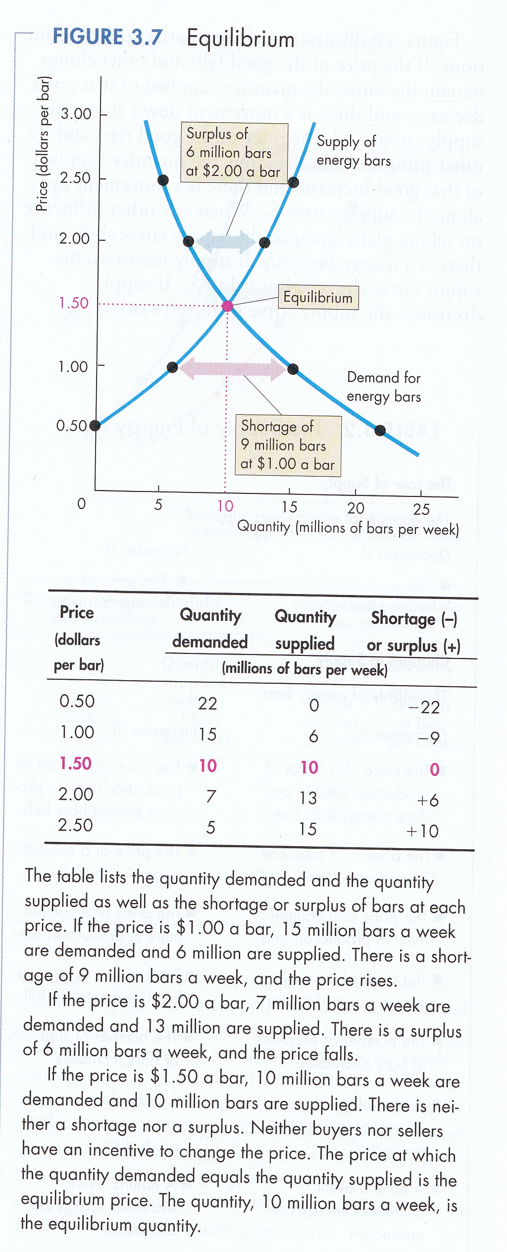
With Market Demand and Supply Curves we generate an ‘X’-shaped
graph
with Demand increasing as price goes down and Supply increasing
as price goes up. There will be a point where the two
intersect. That is called market equilibrium, the point at
which the willingness to buy and the willingness to sell are
equal. Ceteris paribus, this will be a stable
equilibrium, i.e., if all variables remain fixed,
e.g., technology, factor prices, consumer taste, income and
the price of all other goods & services, the price-quantity
equilibrium will be maintained.
Under such fixed conditions if the price
rises, for whatever reason, above equilibrium firms will be
willing to provide more than consumers are willing to buy. A
surplus is created. To eliminate the surplus firms lower price
returning eventually to equilibrium. Similarly, if price drops
below equilibrium consumer demand exceeds supply and a shortage
results. Consumers will then bid up the price until it returns
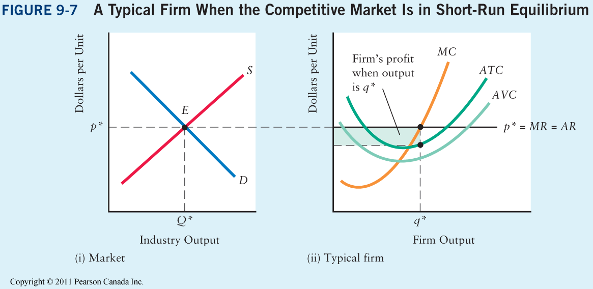
to equilibrium. These are called ‘market forces’ (P&B 4th Ed.
Fig. 4.8; 5th Ed.
Fig. 3.7;
7th Ed Fig. 3.7
R&L 13th Ed
Fig. 9-7).
The actual market outcome – price/quantity –
will, however, depend on the nature of the market. If there are
many, many sellers of identical goods and many, many buyers
there is ‘perfect competition’ and ‘X’ marks the spot. If not,
the outcome reflects the exercise of market power, i.e.,
the ability of one or more buyers or sellers to influence the
final price/quantity outcome.
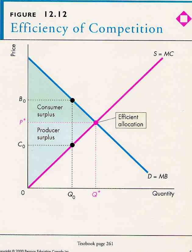
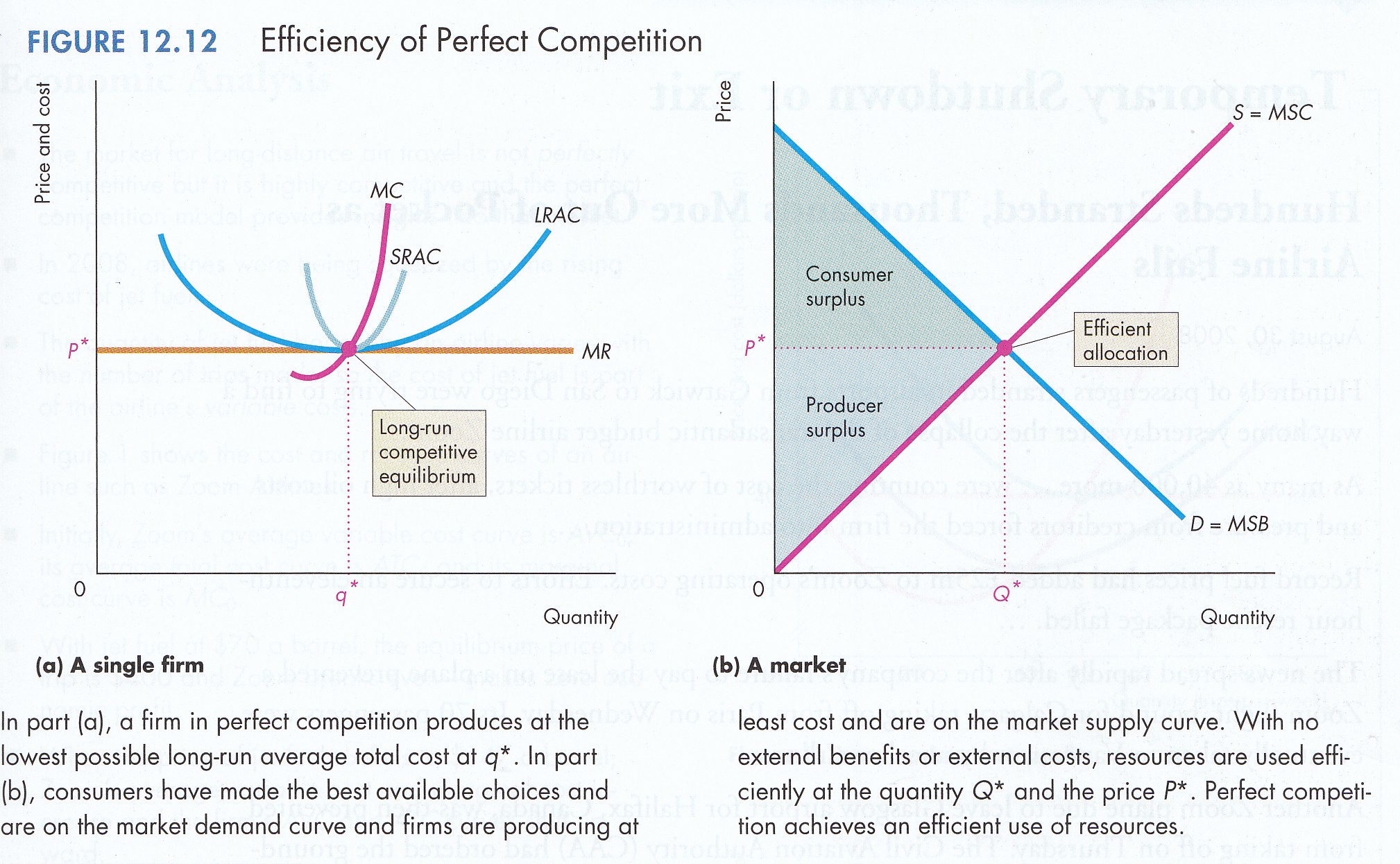
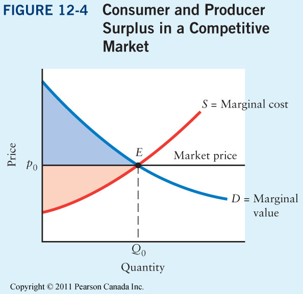
Economic Surplus
In a given market there will be gains
of exchange enjoyed by both consumer and producer. The total
measures the economic surplus.
Consumer
Gains to consumer are called
consumer surplus
(P&B 4th Ed.
Fig. 12.12; 7th Ed
Fig 12.12b; R&L
13th Ed
Fig. 12.4). It
measures the difference between what consumers would be willing
to pay for a given quantity and what they actually pay.
Consumer surplus is measured as the area from market price up to
the demand curve.
Producer
Gains to producers are called
producer surplus
(P&B 4th Ed.
Fig. 12.12; 7th Ed
Fig 12.12b; R&L
13th Ed
Fig. 12.4). It
measures the difference between what firms would be willing to
accept for a given quantity and what they actually receive.
Producer surplus is measured as the area from market price down
to the supply curve.
We now turn to the four major industrial structures: perfect
competition, monopolistic competition, monopoly/monopsony and
oligopoly/oligopsony. In this regard the concentration ratio
can be used as a measure of industrial structure to indicate the
form of competition in a given industry. It is the percentage
of total output supplied by a given number of the largest
firms. In the case of monopoly, for example, one firm supplies
100% of output. In perfect competition and monopolistic
competition the largest 100 firms might contribute just 10 or
20% of total output. In oligopoly/oligopsony the largest 5
firms might account for 50 to 60% or more of total output.
2.2 Perfect Competition
Perfect competition
satisfies four strict conditions:
Anonymity
Consumers are
indistinguishable to producers. Firms have no reason to favor
one consumer over another. The product of different firms is
indistinguishable, one from another, in terms of price, quality
and product differentiation. They are 'homogenous'. Consumers
have no reason to prefer the product of one firm over that of
another. Similarly, any one consumer represents a tiny portion
of market sales and producers have no reason to prefer one
customer over another.
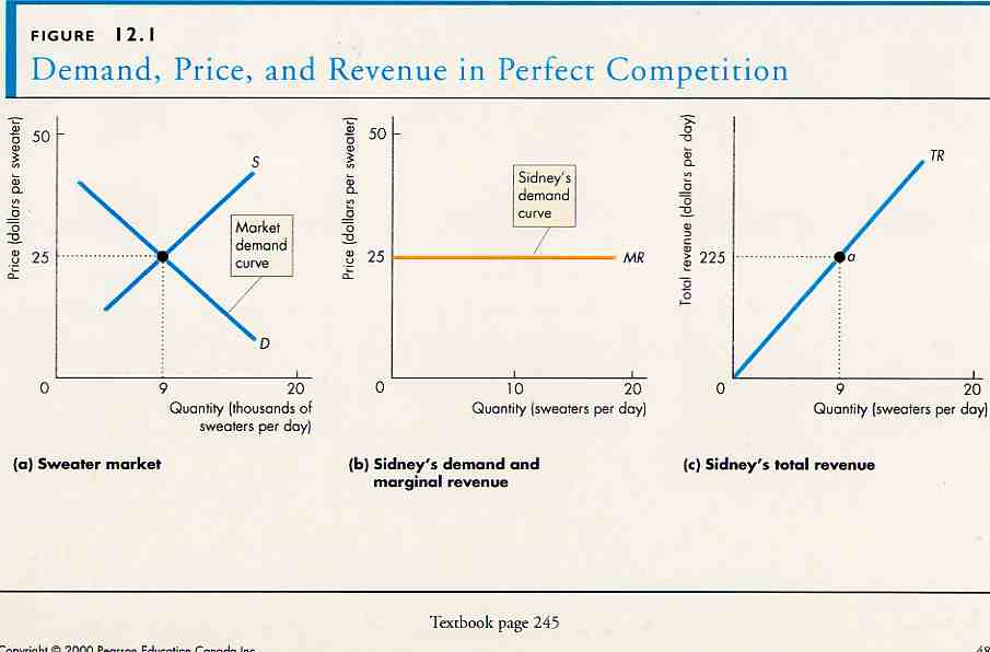
No Market Power
There is a large
number of both producers and consumers. Sales or purchases by
any buyer or seller are small relative to the total volume of
exchange. No buyer or seller can affect price or quality, i.e.,
no one exercises market power. All consumers and producers
respond and adjust only to price signals. The perfect
competitor does not in fact face the market demand curve but
rather market price. The firm is thus a price taker rather than
a price maker. It can sell as much as it wants at market price
but loses all business if it raises the price of its homogenous
output (P&B
4th Ed.
Fig 12.1;
5th Ed Fig. 11.1;
7th Ed
Fig. 12.1).
Perfect Knowledge
Consumers and
producers possess perfect knowledge about price and quality. No
firm can charge more, and no consumer can pay less than the
market equilibrium price.
Free Entry & Exit
Entry and exit from
the market is free for both consumers and producers. There is
an unimpeded flow of resources between alternative uses i.e.,
resources are mobile and move to the use with greatest
advantage in terms of opportunity costs. Firms exit if they
experience ‘economic’ loss. Thereby inefficient firms are
eliminated from the market. Firms enter the market if they
expect to earn economic short-run, and/or, normal
long run profits. On the demand side of the Marshallian
scissors, there are many close substitutes available to
consumers who can easily switch if price, preference and/or
income changes.
2.3 Monopolistic
Competition
Monopolistic competition
satisfies two conditions of perfect competition but fails to
satisfy two others.
Market Niche/Segment
As in perfect
competition there are a large number of sellers. The output of
firms is not, however, considered homogenous by consumers.
Rather they are differentiated. Consider the restaurant
industry. Hamburgers and hot dogs are not the same as pizza or
fried chicken. Some consumers prefer one or the other. In
effect, the market demand curve is disaggregated into distinct
market niches or segments.
Market Power
Within each niche a firm
faces a downward sloping demand curve for its product, i.e.,
they can sell more if they lower price and less if they raise
it. A seller therefore possesses market power, i.e., the
ability to influence the price/quantity outcome, depending on
the elasticity of demand.
Perfect Knowledge
As in perfect
competition, consumers and producers possess perfect knowledge
about price and quality including product differentiation.
Free Entry & Exit
As in perfect
competition, under monopolistic competition entry and exit from
the market is free for both consumers and producers. There are
no barriers to entry or exit. There is an unimpeded flow of
resources between alternative uses i.e., resources are
mobile and move to the use with greatest advantage in terms of
opportunity costs. Firms exit if they experience ‘economic’
loss. Thereby inefficient firms are eliminated from the
market. Firms enter the market if they expect to earn
economic short-run, and/or, normal long run
profits. On the demand side of the Marshallian Scissors,
there are many close substitutes available to consumers who can
easily switch if price, preference and/or income changes.
2.4 Monopoly/Monopsony
Monopoly and monopsony
satisfy one and fail to satisfy three conditions of perfect
competition.
One Seller/Buyer
There is, in the case of
monopoly, no distinction between the firm and the industry,
i.e. there is only one producer. In the case of monopsony,
there is no distinction between the single consumer and the
industry. An example of monopsony is the U.S. Air Force, the
only buyer of B2 bombers.
Market Power
In monopoly, one
producer faces the market demand curve and can accordingly sell
more if it lowers its price and sell less if it raises it. In
monopsony, one buyer faces the market supply curve and can buy
more if it pays a higher price and less if it pays a lower one.
The monopolist is able
to choose the price-quantity combination to maximize its
profits, i.e., it is a price maker. Monopoly power is
mitigated only by competition from substitutes. The closer the
substitutes the less market power is available to the
monopolist. Similarly, the monopsonist can choose which
price/quantity outcome will minimize its cost.
There are, however, two
types of monopoly, i.e., a single price and
discriminating monopolist. The single price monopolist sells
output at the same price to all consumers. The discriminating
monopolist, on the other hand, disaggregates the market demand
curve into individual consumer demand curves. It can then
charge a different price to each individual consumer extracting
the maximum of consumer surplus from each individual consumer.
In effect the discriminating monopolist is able to play on the
willingness of consumers to pay a higher price for a smaller
quantity due to diminishing marginal utility.
Perfect Knowledge
As in perfect competition, consumers and the
monopolist both possess perfect knowledge about price
and quality including substitutes.
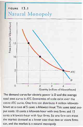
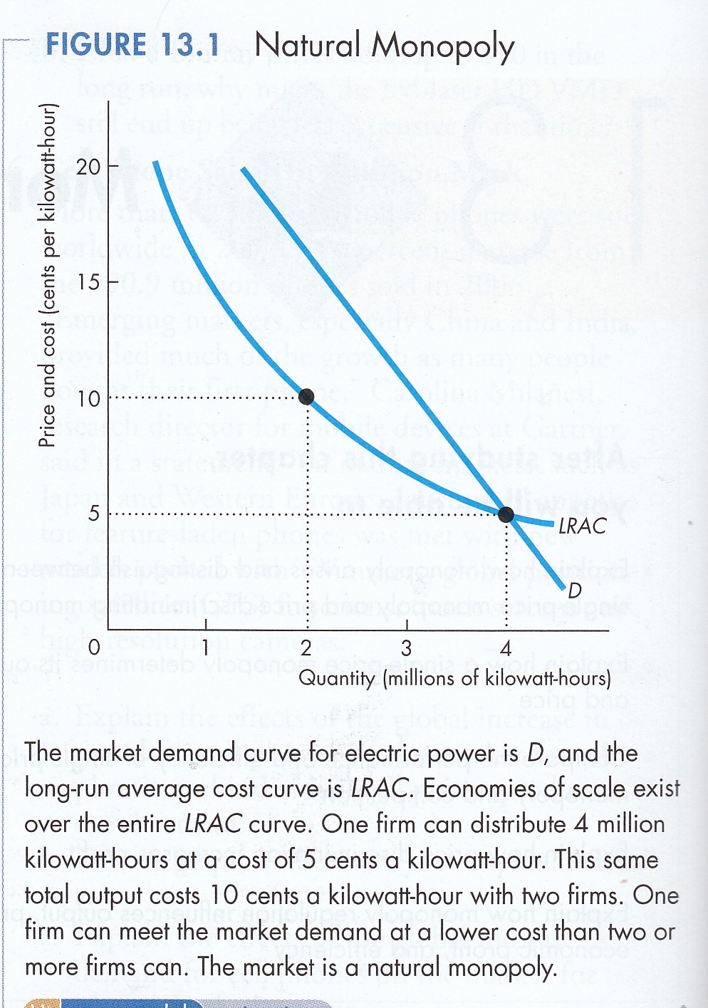
Barriers to Entry
Monopoly exists for one, or more, of four
reasons. First, a firm may become a monopolist because
economies of scale allow the monopolist reach an output level
sufficient to supply the entire market at minimum average cost
per unit. This is a natural monopoly (P&B 4th Ed
Fig. 13.1; 5th Ed. Fig. 12.1;
7th Ed Fig. 13.1; R&L 13th Ed not displayed).
Second, one firm may control the entire supply of a basic
input. An example would be a mineral critical to production of
the good in question and the monopolist owns the only mine
producing that input. Third, a firm may acquire control
over a product due to an intellectual property right -
copyright, patent, registered industrial design or trademark -
granted by the State. Fourth, a firm may become a
monopolist because government awards an exclusive market
franchise, e.g. electric power, water supply, etc.
A monopolist is not, however, entirely
insulated from the economy as a whole. All commodities are
rivals for the consumer’s limited income. The closer are
substitutes, the greater the moderating influence on a
monopolist. The threat of entry by outsiders interested in
gaining some of the monopolist’s excess profits also serves to
moderate pricing behavior, e.g. the threat that cable
companies could offer telephone service will limit the pricing
of a telephone monopolist.
2.5 Oligopoly/Oligopsony
Oligopoly/oligopsony
satisfies none of the conditions of perfect competition.
Few Large Sellers/
Buyers
In the case of
oligopoly, there is a small number of large firms that dominate
the industry. Often these majors are surrounded by a
competitive fringe of smaller firms usually operating in
distinct market niches or segments. The action of a major
producer is perceptible to rivals, i.e. there is
interdependency of sellers whereby an action by one results in
reaction of others. Furthermore, the output of producers is not
seen as homogenous by consumers. This is often the result of
successful branding. Thus each major enjoys a certain market
share based on product differentiation.
In the case of
oligopsony, there is a small number of large buyers that
dominate the industry. Often these majors are surrounded by a
competitive fringe of smaller buyers, again usually operating in
distinct market niches or segments. The action of a major
buyer is perceptible to rivals, i.e. there is
interdependency of sellers whereby an action by one results in
reaction of others. An example of an oligopsony are the ‘big
box stores’ like Walmart, Target, Safeway, etc. Due to the
scale of there purchases they can influence the price/quantity
outcome at which they buy from suppliers.
Market Power
Due to economies of
scale, product differentiation like
branding as well as process/product innovation, oligopolists
exercise market power in determining the equilibrium
price/quantity relationship in a market.
Imperfect & Asymmetrical Knowledge
Unlike perfect competition, consumers as well
as oligopolists and oligopsonists do not possess perfect
knowledge. Specifically, they do not know how or when other
players will react to the actions of a major. For example, if
Ford Motor Company offers zero percent APR (above prime rate)
financing will Toyota respond the same way or choose an
alternative strategy like a long warranty? This opens up
the question of asymmetrical information including issues such
as insider trading.
Barriers to Entry
Oligopoly/Oligopsony also exhibit barriers to
the entry of new firms. Economies of scale can thus inhibit
entry. Product differentiation through branding can also make
it difficult for a new firm to enter the industry. And, as will
be seen under 4. Performance, the excess or economic profits
earned by oligopolists allow them to invest in advertising –
branding – as well as product and process innovation. A lean,
mean, perfectly competitive firm can afford neither.
2.6
Integration/Conglomerateness
In Microeconomic
theory we are dealing with a single product, profit maximizing
firm. In Industrial Organization we are dealing with real world
industrial structures which include vertical, horizontal and
conglomerate integration.
Vertical integration
unites under one owner a number of plants engaged in successive
processes or stages of production. An example is a vertically
integrated oil company co-temporally engaged in exploration,
production, refining and retailing. Horizontal integration
unites under one owner a number of plants engaged in the same
processes or stage of production. An example is a multi-plant
firm engaged in metal fabrication. Output becomes an input to
other industries which combine them with yet other inputs in
their own production process.
Conglomerateness, on
the other hand, involves diversification beyond the boundaries
of any given industry. Conglomerate mergers were the rage in
the United States during the 1960s because anti-trust policies
inhibited significant concentration due to either vertical or
horizontal mergers. With fat profits in their corporate pockets
many firms argued that ‘management’ was the ultimate economic
resource. If one could manage steel then one could manage
airlines, chocolate bars or any other business. In effect,
local knowledge was considered less important than management in
building a business success. With the notable exception of
General Electric most conglomerate mergers of the ‘60s failed.
2.7 Government Intervention
Government
intervention is a pervasive structural characteristic of all
industries and markets. The form and nature of that
intervention takes varying forms. Bankruptcy, environmental,
financial, health & safety, incorporation, labour and protection
of persons & property are just some of the areas in which
government plays an active role in every industry. I will first
argue that equity provides both the legal and economic rationale
for governmental intervention. I will then highlight non-market
forces unleashed by certain forms of governmental intervention,
specifically price setting.
Anti-Trust & Combines in a Global
Economy
from 50s to Globalization
Equity & Regulation
Courts of Common Law are one of the great
contributions of the Anglosphere. Formally beginning in the
reign of Henry II in the 12th century, Common Law, unlike
Statutory and Regulatory Law, originates in the Anglosphere.
Two things make Common Law different. First, judges may
“make” Law by setting precedents. The body of precedent is
called “common law”. If a similar case was resolved in the
past, a current court is bound to follow the reasoning of that
prior decision on the principle of stare decisis. The
process is called casuistry or case-based reasoning. If
a current case is different, however, then a judge may set a
precedent binding future courts in similar cases. Casuistry
must begin again, however, if changes or amendments to Statutory
or Regulatory Law negate the precedent.
Second,
Common Law is rooted in trial by jury, i.e., one’s
peers. This is a fundamental civil right in the Anglosphere in
criminal law. By contrast, the European Civil Code tradition is
based on trial by judge/prosecutor, i.e., the police and
judicial functions merge in one office. On the other hand, the
impresciptible
moral rights of authors are recognized
under Civil Code but not Common Law. Similarly there is the
treatment of torts, i.e., non-contractual rights and
obligations. Under Common Law they are treated by precedent and
trial ‘attorneys’ in the U.S.A. enjoy a large practice. Under
Civil Code such questions are answered by principle, somewhat
like equity in the Anglsophere.
However, at the same time the Common Law
arose during the resign of Henry II another unique Anglosphere
juridical institution emerged – Equity. It was not guilt or
innocence but fairness of punishment before the King. This is
the root of Equity – a separate and distinct strand of
jurisprudence parallel to the Common Law of precedent.
Over time responsibility for hearing calls
for mercy was transferred to the King’s Lord Chancellor and a
court of his own – the Court of Equity also known as the Court
of Conscience or of Morality. In fact until Sir Thomas More (a
lawyer) became Chancellor in 1529, all had been men of the
cloth. Two aspects of Equity played a critical role in the
Sovereign’s ability to control his vassals. These were trusts
and tenant-landlord disputes. Trusts (from which modern
charities and financial trusts evolved) generally concerned
widows and orphans left to the mercy of a local lord. The most
famous is Lady Marion of the Robin Hood legend who was an orphan
and ward of the King. With respect to tenant-landlord disputes,
Equity balanced the feudal local lords by judiciously connecting
the King to his subjects. This was called the ‘rent bargain’ by
J.R. Commons (1924). It stabilized the social system of
post-Conquest England.
While Magna Carta (1215) and
subsequent developments increasingly limited the King, Equity
and Common Law continued to develop as parallel systems of
courts with precedence given to Equity. It was not until 1873
in the United Kingdom that the two systems of courts merged,
i.e., cases at Equity could be heard by the same courts that
ruled under Common Law. Nonetheless the two strands of
Anglosphere jurisprudence continue to this day in all Common Law
countries with Equity retaining precedence.
The economic concept of Equity arguably
derives from legal Equity. In fact the Chancellor of the
Exchequer exercised a concurrent jurisdiction in Equity with the
Lord Chancellor’s Court. There are three economic definitions
of Equity, each reflecting its historical roots. First,
there is Equity as the capital of a firm which, after deducting
liabilities to outsiders, belongs to the shareholders. Hence
shares in a limited liability corporation are also known as
equities. This links back to the historical treatment of trusts
under Equity.
Second,
there is Equity as ‘fairness’. While often used with reference
to taxation it is a general economic concept. With respect to
taxation Equity has three dimensions: horizontal, vertical and
overall burden. Horizontal Equity refers to ‘like treatment of
like’. Vertical Equity refers to ‘unlike treatment of unlike’.
Overall Equity refers to the accumulated impact of all forms of
taxation. Crudely, it is the difference between earned and
disposable income after all taxes – income, excise, sales, et
al.
Equity thus provides the legal and economic
rational for government intervention in the economy. Such
interventions include, of course, the Corporations Act and
Bankruptcy Act. It also justifies anti-trust and anti-combines
legislation to counter the exercise of market power.
Non-Market Forces
We have seen that if a competitive
market is allowed to operate an equilibrium price/quantity
outcome will result from the interplay of market force. If
price is too high, Supply exceeds Demand and a surplus is
created. To get rid of the surplus producers must lower their
price, eventually to equilibrium. Similarly, if price is below
equilibrium then Demand exceeds Supply and a shortage is
created. Consumers wanting the good bid up its price back to
equilibrium.
What happens, however, if government
intervenes and does not allow market forces to function? I will
now consider such price setting intervention in agriculture,
housing, labour, prohibited goods and taxation.
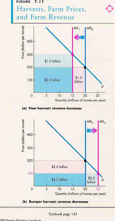
Agriculture
Agriculture is subject to significant
fluctuations in supply yet a relatively inelastic demand, people
have to eat. We begin by assuming only domestic production is
involved. In any given year, the supply is fixed and perfectly
inelastic, a harvest is the harvest is the harvest. In an
unregulated market (P&B 4th Ed.
Fig. 7.11; 5th Ed. Fig. 6.11; 7th
Ed not displayed;.
R&L 13th Ed not displayed), a bad harvest shifts supply
to the left. This raises prices and will actually increase
revenue to the farmer. A bumper crop, on the other hand, will
shift supply to the right, lower prices and reduce farm income.
Many agricultural commodities can be
stored, that is placed in inventory. Inventories serve to
stabilize prices between growing seasons. Without inventories
the above situation applies, that is a good harvest lowers
prices, a bad harvest raises prices. Inventories reduce these
price fluctuations (P&B 4th Ed.
Fig. 7.12; 5th Ed. Fig. 6.12; 7th
Ed not displayed;.
R&L 13th Ed not displayed). A good harvest can be used to
increase inventories, that is, not all output goes to market and
price decreases are moderated. In the case of a bad harvest,
inventories are sold, thereby increasing supply and reducing
price increases.
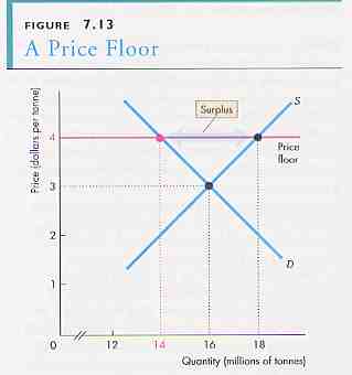
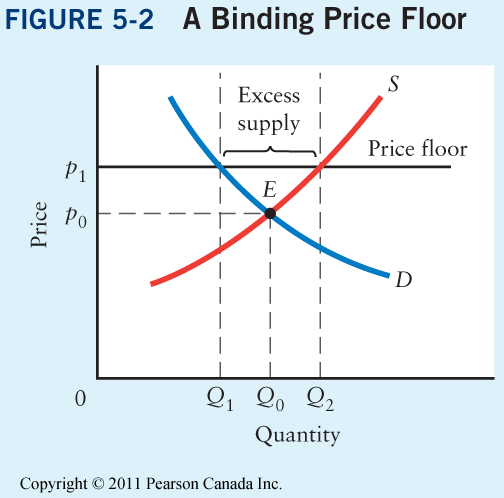
A price floor acts like a minimum
wage. If the floor is less than market equilibrium, it has no
effect. If it is greater than equilibrium price it will create a
demand gap between the larger amount suppliers are willing to
provide at the floor price, and the quantity consumers are
willing to buy (P&B 4th Ed.
Fig. 7.13; 5th Ed. Fig. 6.13; 7th
Ed not displayed;.
R&L 13th
5-2).
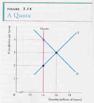
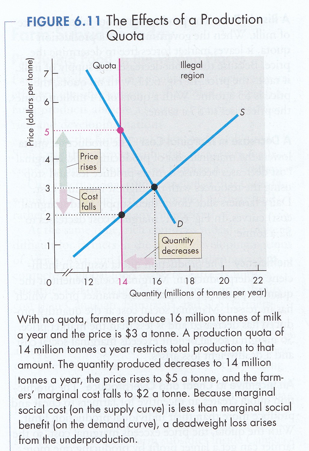
Quotas (on eggs, grain, beef, etc.)
act like a perfectly inelastic supply curve (P&B 4th Ed.
Fig 7.14; 5th Ed. Fig. 6.14; P&B
7th Ed Fig. 6.11;.
R&L 13th
5-8).
If the quota output is less than equilibrium output the price
will be higher and the supply lower. This creates a supply gap
where producers have an incentive to exceed their quota. This
can lead to increased
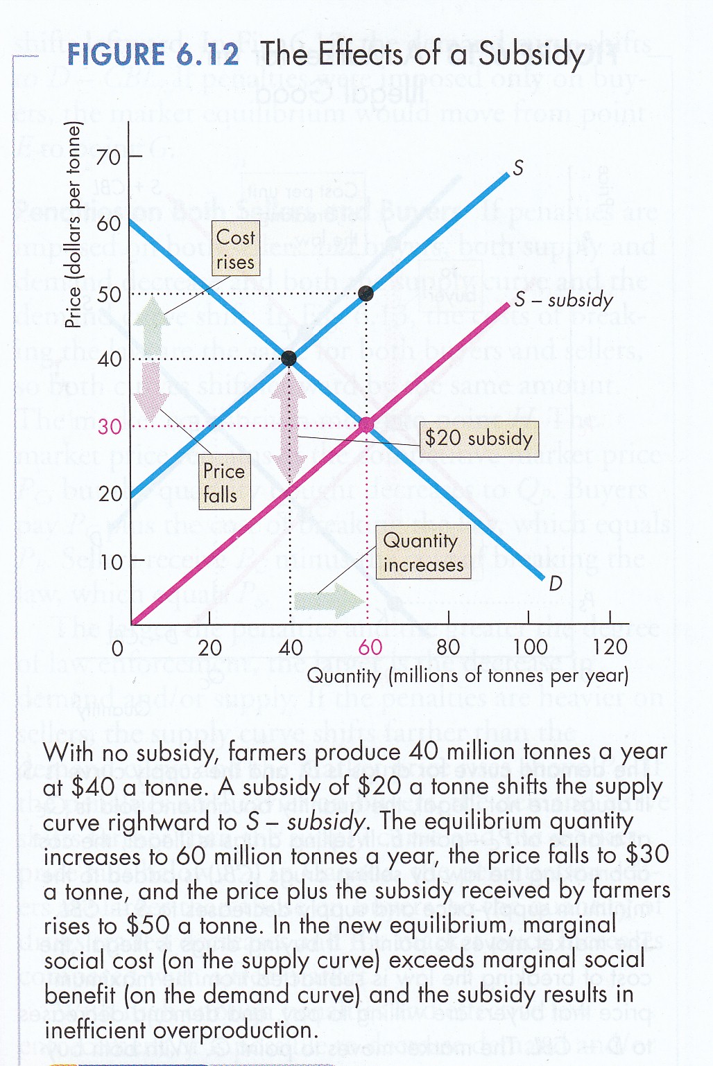
Subsidies act like a reverse tax (P&B
4th Ed.
Fig. 7.15;
5th Ed. Fig. 6.15; P&B
7th Ed Fig. 6.12;
R&L 13th Ed not displayed). The tend to shift the supply
curve to the right. Output increases and prices fall. Such
'supply-side' subsidies financially reward increased production
by offering subsidies per bushel of output or per acre planted.
This approach has led to a frightening subsidy spiral. In
effect, production subsidies reduce the final price of farm
output below the cost of production. This, in turn, means that
even efficient farmers cannot earn enough to maintain
operations. This, in turn, leads to more subsidies that lower
prices further. And, so on and so on and so on...
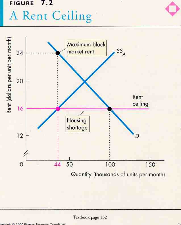
Housing
Part of the short-run adjustment
process involves price, that is, if demand exceeds supply,
prices will tend to rise. In the case of rental property, which
tends to be the type of housing available to the poorer members
of a community, a price rise takes the form of rent increases.
If government decides for reasons of vertical equity (unlike
treatment of persons in unlike situations) that the poor need to
be protected from rent increases (or for political reasons,
there are more poor voters than landowners) then it may impose
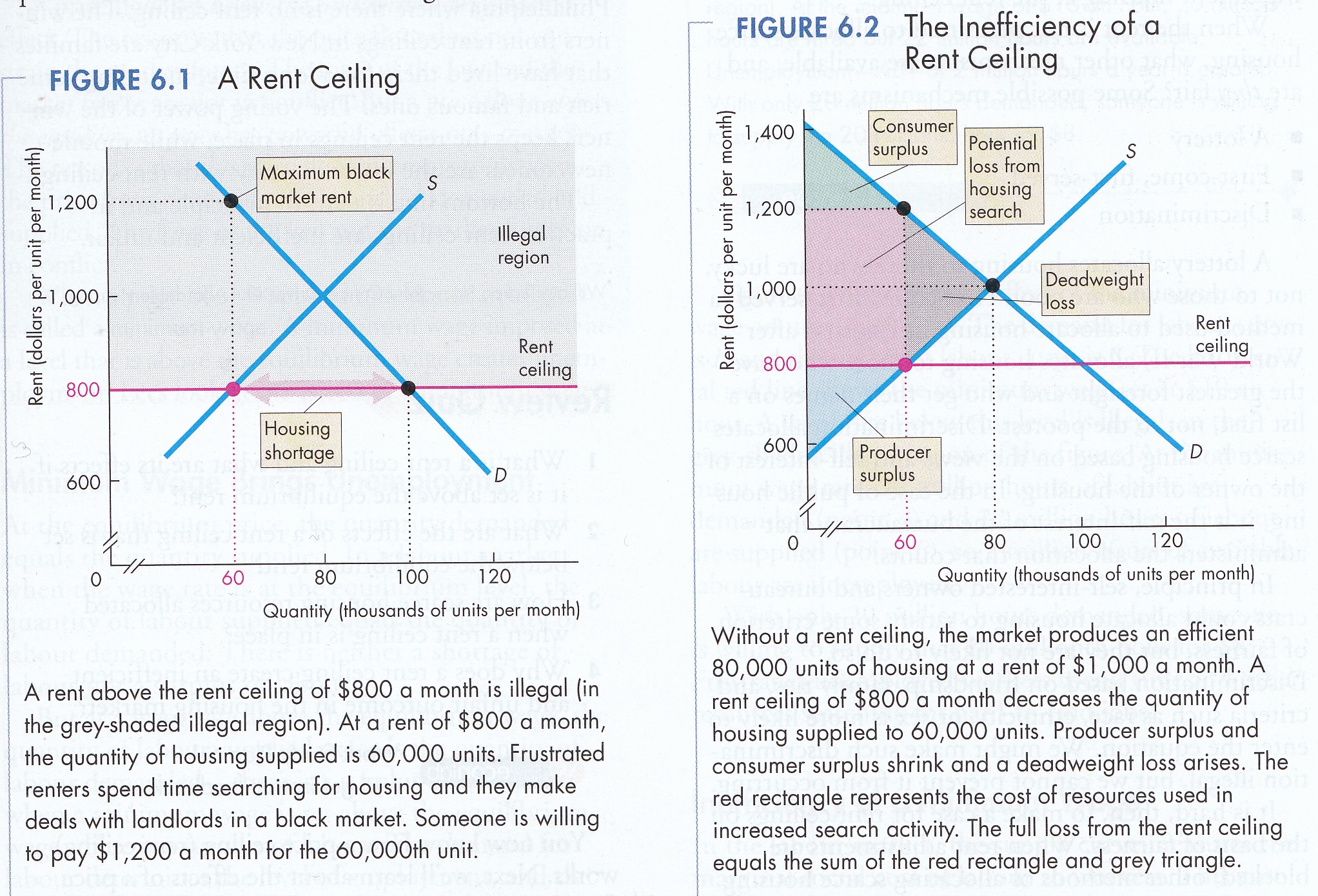
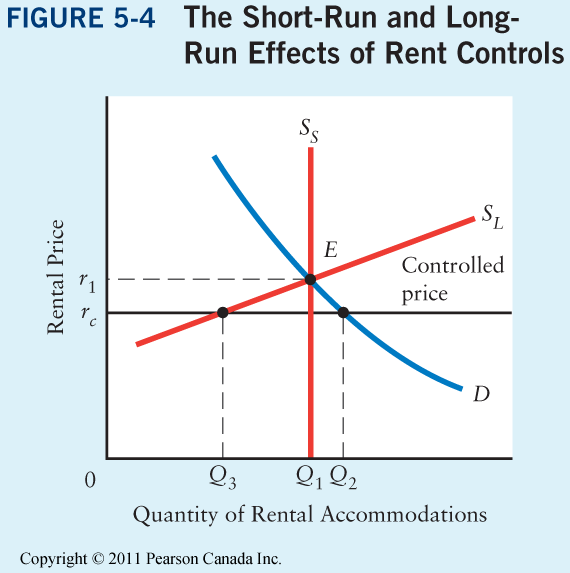
rent controls in the form of a rent ceiling (P&B 4th Ed.
Fig. 7.2;
5th Ed. Fig. 6.2; 7th Ed
Fig. 6.1 & Fig. 6.2;.
R&L 13th
5-3 &
5-4).
In effect, rent control imposes a
price which is less than that determined by the market. This
means that demand (the willingness of consumers to pay) exceeds
the supply (the willingness of producer to supply). This results
in a housing shortage. Because demand exceeds supply yet price
can not increase other forms of behaviour take the place of a
price increase. For example, given a shortage:
i - consumers must search harder and
harder to find supply when it does become available. Search
activity is costly; and/or,
ii - consumers will 'bribe' supplier,
for example, by paying more 'on the side'; by accepting little
or no maintenance or support services; by accepting 'run down
conditions'.
The effect of rent control is to
reduce the return to suppliers. If they cannot cut back
production directly they may do so indirectly. First, new rental
accommodation will not be built which, if population continues
to grow, accentuates the shortage. Second, existing rental
property will be allowed to 'run down', eventually into 'slum
condition'. With excess demand and a fixed price, the supplier
can recoup his or her opportunity cost by running the building
down until it is uninhabitable, then tear it down and build
private homes or condos for sale on an open and competitive
market without price controls. This again accentuates the
housing shortage.
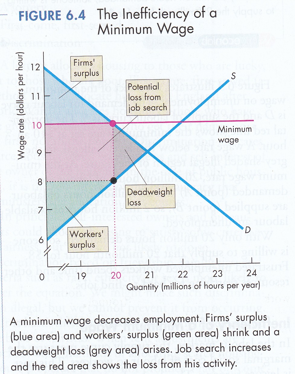
Labour
Low wages for unskilled labour may
create a question of vertical equity (or political reasons).
Government may decide that with such low wages unskilled workers
cannot support themselves, their children and/or other
dependents above the 'poverty line'. Accordingly government may
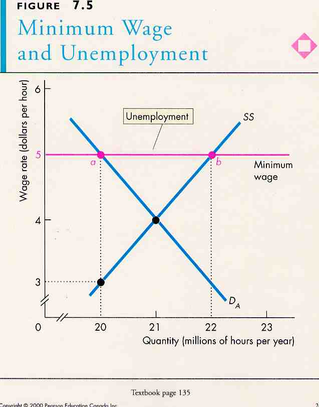
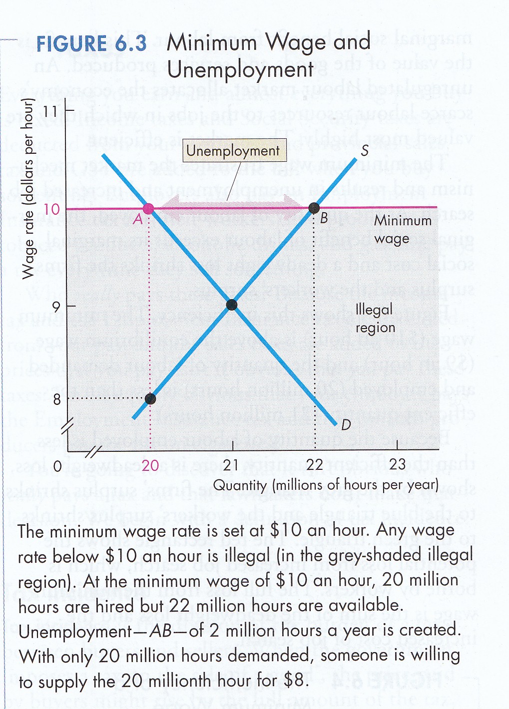
intervene by establishing a 'minimum wage rate'.
If this rate is below market
equilibrium rate such a minimum has no real effect. If, however,
it is above the market equilibrium price (P&B 4th Ed.
Fig. 7.5;
5th Ed. Fig. 6.5; 7th Ed
Fig. 6.3
&
Fig. 6.4;.
R&L 13th p. 103, no JPEG available) the supply of willing workers
exceeds the demand of producers. As in the case of rent
controls, if the price cannot adjust, other forms of behaviour
will evolve. For example, some workers will offer to work some
hours 'off the books'.
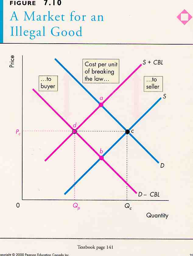
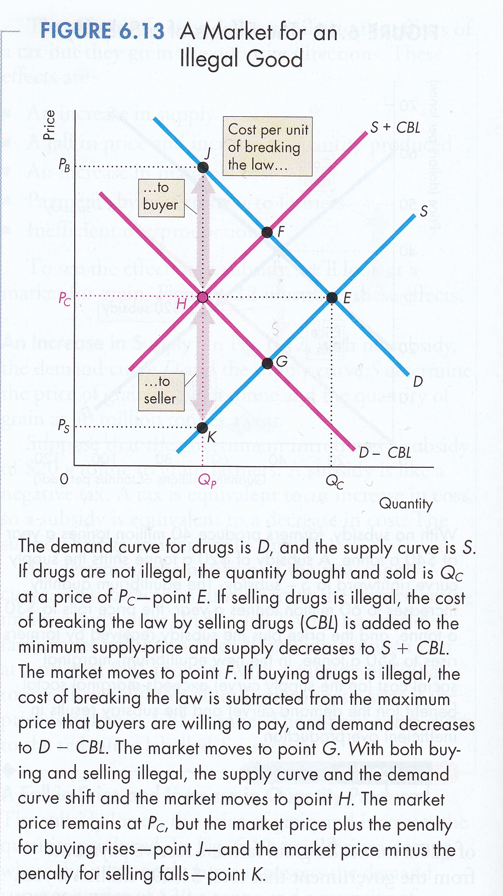
Prohibited Goods
While some goods like recreational
drugs are illegal and hence prohibited, a market exist. To
understand the effect of prohibition, we begin with market
equilibrium assuming no prohibition (P&B 4th Ed.
Fig. 7.10;
5th Ed. Fig. 6.10; P&B
7th Ed
Fig. 6.13;
R&L 13th 5-3). A prohibition affect both
demand and supply. It imposes penalties, that is costs, on both.
The effect is to shift the supply curve up to the left and shift
the demand curve down to the left.
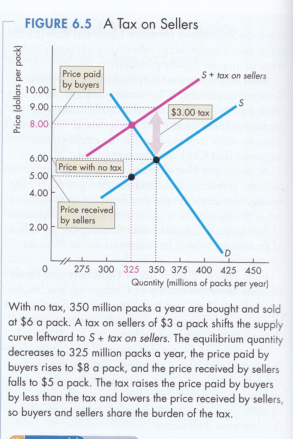
Taxation
To finance public spending (a
pleasure), government must raise revenue through taxes (a pain).
This pleasure/pain of public finance is described in the
Introduction: The Pleasure & Pain of Public Finance to my paper
"A
Radical Analysis of 'Personal' Taxation."
An increasingly important source of tax revenue is sales tax,
for example, the GST and provincial sales tax. The question
arises: who pays Is it the consumer or the producer or both?
Consumer demand does not change if a
sales tax is imposed. The demand curve reflects the quantity of
a good or service consumers are willing to buy at a given price.
If the price goes up, one slides up the demand curve; if the
price goes down, one slides down the demand curve - all things
being equal. Accordingly, to the consumer the real price of a
good is its retail price plus any associated taxes.
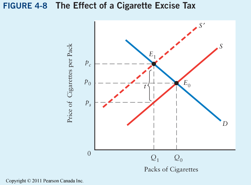
A sales tax does, however, shift the
supply curve up to the left. Producers are willing to supply a
certain quantity of goods or services if the receive a given
price. With sales tax, such goods and services are offered for
sale at a higher price (P&B 4th Ed.
Fig. 7.6;
5th Ed. Fig. 6.6;
7th Ed Fig. 6.5;
R&L 13th Ed Fig.
4-8
&
4-9).
The supply curve shifts and a new equilibrium is established at
a higher price and a lower quantity than before the tax.
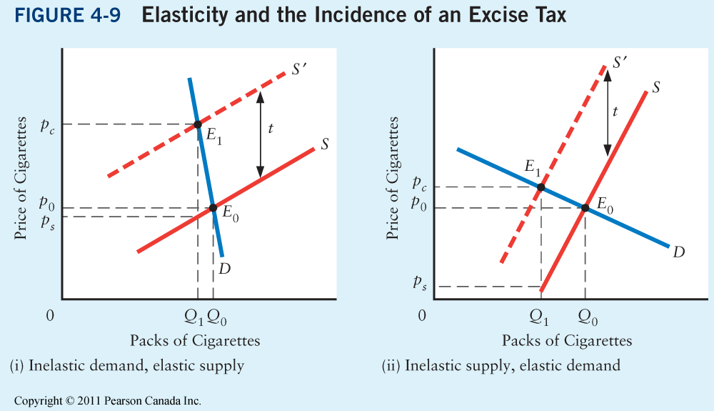
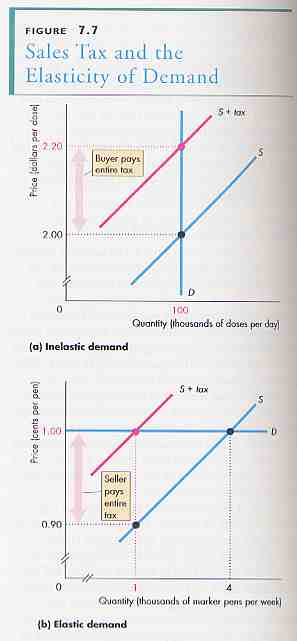
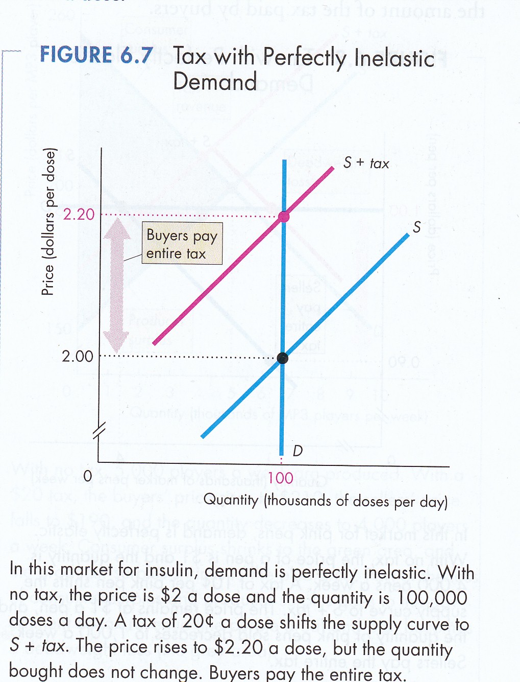
As to who pays the tax, the answer
depends on the elasticity of supply and demand. If there is
perfectly inelastic demand, for example for a 'necessity', the
demand curve is vertical (P&B 4th Ed.
Fig. 7.7a;
5th Ed. Fig. 6.7;
7th Ed Fig. 6.7)
In this case the consumer pays the full tax. If, on the other
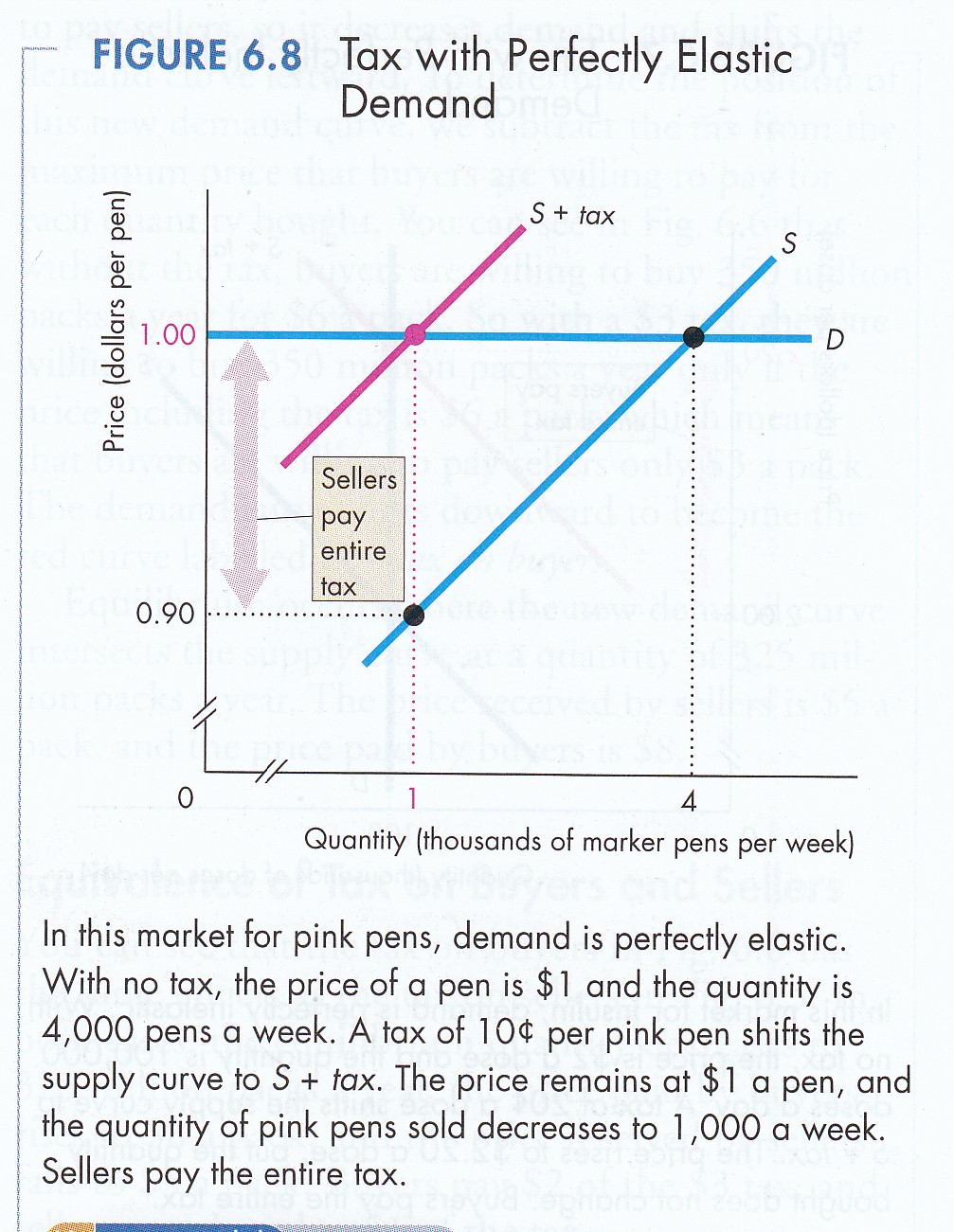
hand, demand is perfectly elastic ((P&B 4th Ed.
Fig. 7.7b;
5th Ed. Fig. 6.7;
7th Ed Fig. 6.8;
R&L 13th Ed Fig.
4-8
&
4-9),
then the producer pays the whole tax.
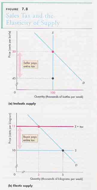
In the case of supply elasticity, the
situation is reversed (P&B 4th Ed.
Fig. 7.8;
5th Ed. Fig. 6.8;
7th Ed Fig. 6.9).
If supply is totally inelastic, that is the supply curve is
vertical, then the supplier bares the full tax. If supply is
perfectly elastic, however, the consumer will pay the tax