Microeconomics
Macroeconomics
SISTERetrics
SITES
Compleat World Copyright Website
World Cultural Intelligence Network
Dr. Harry Hillman Chartrand, PhD
Cultural Economist & Publisher
©
h.h.chartrand@compilerpress.ca
215 Lake Crescent
Saskatoon, Saskatchewan
Canada,
S7H 3A1
Launched 1998
|
Microeconomics 3.0 Supply (cont'd)
|
|
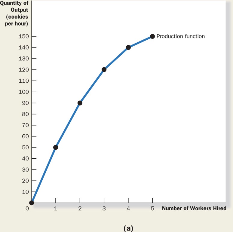
1. Production Function (MKM C13/279-81; 260-2; 285-287; 265-267) In symbolic logic the production function of a firm is: (7) Q = g (L, K, N) where: Q = output g = some function reflecting ‘know-how’ in combining inputs to produce output, a.k.a., technology L = labour K = capital N = natural resources that can be enabled to serve human purpose.
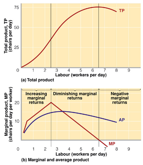
The production function is time sensitive. However, the short- and long-run in economics is measured not in chronological time but in functional time, e.g., how long it takes to build a new plant. Thus the long-run in the restaurant industry is chronologically shorter than in the steel or nuclear industries but both are functionally the long-run in their respective industries. There are three types of time periods. We will graph only in two dimensional space with K and L considered. i - Very Short-Run In the very short run, or what Marshall called ‘the market period’, output is fixed. All factors of production are fixed – labour, capital and natural resources. The very short-run supply curve is vertical and does not change with price. An example is the farmers’ market where produce is brought into the city from the farm for sale. No more produce is available. What is on hand is all that can be sold, no matter price. (8) Q = g (L, K) where K, L & Q are all fixed ii - Short-Run (MKM C13/288-9; 268-70) In the short-run at least one factor of production is fixed, generally capital plant and equipment (MBB Fig. 7.2). More or less labour and natural resources can be employed and output increased or decreased. (9) Q = g (L, K) where L is variable K is fixed Q is variable With capital fixed and labour variable in the short run we can graph the production function as an 'S' shaped curve (MKM Fig. 13.2). Initially as labour is added its marginal product increases up to about 2.5 units in the graph (increasing MPL) and then it begins to decrease from 2.5 up to 6.5 units (diminishing MPL) becoming zero at the peak of the curve and then turns negative (negative MPL). No profit maximizing firm will expand by hiring more labour if total output is decreased, i.e., beyond the peak of the production curve. There are, of course, some firms such as State owned companies in China that are not profit maximizers but rather employment maximizers. Why does MPL eventually decline and become negative. The simple answer is that capital is being spread thinner and thinner among more and more workers reducing their marginal product. In addition more and more workers means increased congestion and complexity. This is called the law of eventually diminishing marginal product which has significant implications for the costs of a firm as output rises. It parallels the law of eventually diminishing marginal utility in Consumer Theory, i.e., eventually the marginal utility of a good declines and becomes negative, too much of a good thing makes you sick. The marginal product of labour, i.e., the additional output generated by employing one more unit of labour is measured by the slope of the production function. The average product of labour, or the average output of all workers, is measured by the slope of a ray, i.e., straight line, from the origin where it intersects the production function. It should be noted that some rays will intersect the production function at two points. At each of these two points average product is the same. As will be seen this has significant implications for the shape of the marginal and variable costs curves of a firm, specifically their 'U' shape. As will be seen, if we know the cost of labour we can calculate the marginal cost of an additional unit of output and the average variable cost of any given level of output. iii - Long-Run (MKM C13/288-9; 268-70; 293-296; 273-274) In the long-run all factors of production are variable – capital plant & equipment, labour and natural resources. (10) Q = g (L, K) where L is variable K is variable Q is variable As noted previously modern microeconomic theory began with demand and the constrained maximization of utility by the consumer demonstrated using indifference curves and budget constraint. Initial attempts to explain production adopted the same basic mechanism with one important change: measurement of output is cardinal. That is we can, unlike utiles, count the exact number of units being produced. The firm thus wants to maximize output (Q). The firm, however, faces a constraint: the cost of inputs or factors of production. In symbolic logic, this cost constraint is: (11) C = PLL + PKK where L = labour K = capital PK = price of capital PL = price of labour Assuming all factors are infinitely divisible then different levels of Q can be produced using different factor combinations. This generates an isoquant a curve representing a constant level of output all along its run (R&L 8A-1; M&Y 10th Fig. 8.2). The slope of the isoquant is the marginal rate of technical substitution (MRTS) of capital for labour maintaining the same Q. In symbolic logic it is (12) MRTS = MPL/MPK where MPK = marginal product of capital MPL = marginal product of labour There are theoretically an infinite number of isoquants rising to higher and higher levels of output (R&L 8A-2). They are convex to the origin (opening away) due to the Law of Diminishing Marginal Product which states that as one factor is given up in favour of another eventually marginal product of the increasing factor will decrease. While the firm wants to maximize Q it faces a cost constraint. For a given cost a maximum amount of capital or labour can be bought illustrated by the intercepts of the x- and y-axis. Its slope is the relative cost of the two factors or in symbolic logic is: (13) Cost Ratio = CL/CK As with the budget constraint price ratio by convention the cost ratio is the inverse of the slope of the resulting cost constraint curve. The curve shows all combinations of K and L that can be bought for a specific cost (R&L 8A-3; M&Y 10th Fig. 8.2). Maximum Q for a specific cost is achieved where the cost constraint just touches or is tangent to the highest attainable isoquant. At that point, the slope of the cost constraint equals the slope or MRTS of the isoquant. (14) MRTS = MPL/MPK = - (CL/CK) and (15) MPL/CL = MPK/CK where dollar-for dollar the marginal product of an additional unit of L is equal dollar-for-dollar to the marginal product of an additional unit of K iv - Expansion Path As with consumption and the Income Consumption Curve, if we relax the cost constraint while holding factor prices constant, a new cost constraint with the same slope (CL/CK) is created and a new equilibrium established. Repeating this process a locus of point is created all of which satisfy the equilibrium conditions (MPK/CK = MPL/CL) forming the expansion path for the firm (M&Y 10th Fig. 8.18). This initial attempt to plot the supply curve of the firm was judged inadequate for the simple reason that factors of production especially capital are not infinitely divisible but rather ‘lumpy’ particularly in the short-run. A new approach was required that focused on the short-run behavior of the firm.
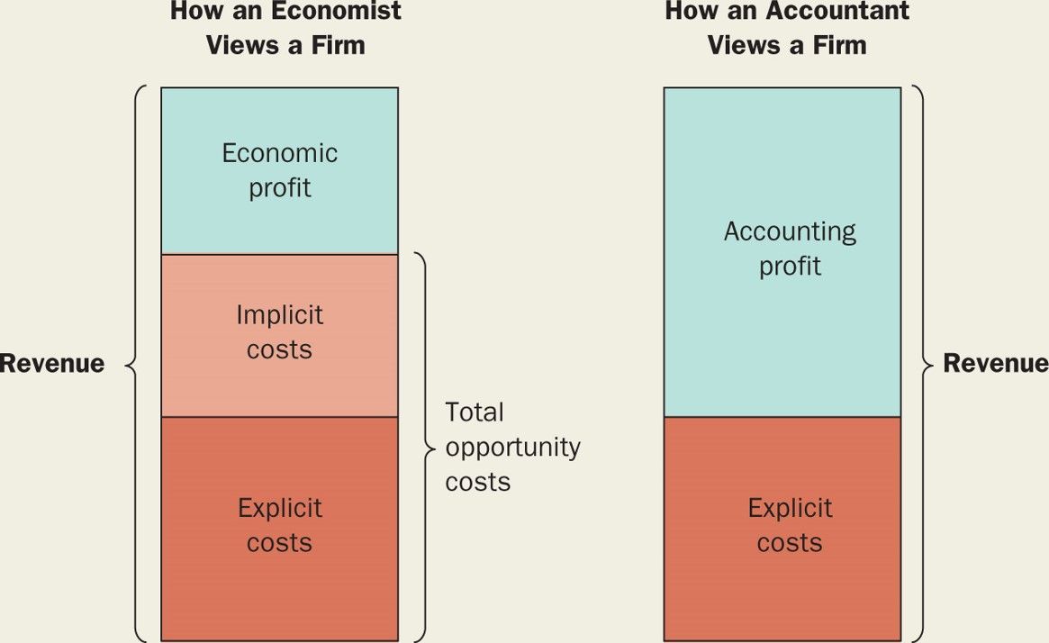
2. Cost (MKM C13/281-91; 262-271; 287-296; 267-274) i - Opportunity Cost Economic choice involves how to satisfy infinite human wants, needs and desires with scarce resources. It requires a choice between alternatives, e.g., a pensioner choosing food or medicine. The choice of the best alternative means the next best alternative is not chosen. Put another way, the cost of choosing one possibility is the next best alternative foregone. This is called ‘opportunity cost’. All economic costs are opportunity costs even those not expressed by market prices.
While
for convenience one usually measures opportunity cost in dollars it
actually involves real alternatives foregone. Thus for a firm,
the opportunity cost of producing (OCP) a good (and therefore opportunity
cost of employing factors of production) is the next best alternative action.
There are two components to a firm’s OCP : explicit and implicit costs ii - Fixed, Variable &Total (MKM C13/282-3; 264-5; 288-290; 268-270) Assuming one factor of production is fixed (usually capital) then we are in the short-run and can identify three types of costs measured in three different ways. In the short-run a firm can produce different levels of output but only by varying variable inputs. Accordingly the firm has three distinct types of costs: a) fixed costs associated with the fixed factor of production - usually K but in the knowledge industries often L or 'the talent'. Fixed costs must be paid no matter the level of output, i.e. even if the firm shuts down fixed costs still have to be paid; b) variable costs associated with variable factors of production - usually L. Variable costs rise and fall according to how much of the variable factors are employed. The higher the level of production, all things being equal, the higher the variable costs; and, c) total costs that include all fixed and variable costs or TC = TFC + TVC (MKM Fig. 13.5).
iii -
Average, Marginal & Total
[MKM
C13/283-9;
290;
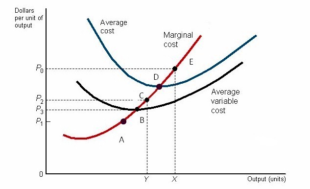
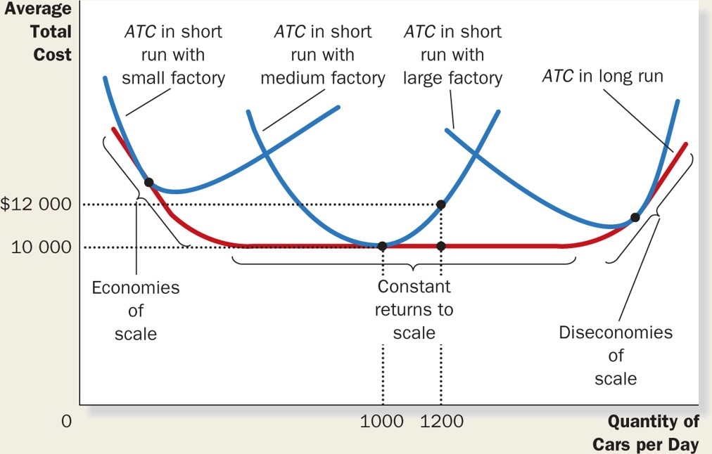
269-270) In turn, for each type of cost at every level of production, average costs can be calculated: a) Average Fixed Cost (AFC) = fixed cost per unit output. AFC will decline as output increases as the fixed cost is spread over a larger and larger level of output; b) Average Variable Cost (AVC) = variable cost per unit output. The distance between the AVC curve and the TC curve will tend to narrow as output increases because AFC declines as output increases; and, c) Average Total Cost (ATC) = fixed (AFC) + variable (AVC) cost per unit output. In turn, for each level of production, marginal cost can be calculated from the cost associated with one additional unit of output (M&Y 10th Fig. 8.10). Average total and marginal cost can also be calculated from the total cost curve. Average total cost can be derived from the slope of a straight line or 'ray' drawn from the origin to any point on the total cost curve. Marginal cost can be derived from the changing slope of the total cost curve itself. Marginal cost (MC) will initially decline as output increases but eventually, assuming at least one fixed factor of production, the Law of Eventually Diminishing Marginal Product/Return sets in and marginal cost begins to rise. The MC curve will cut the average cost curve (AC) at its lowest point. Thus as long as MC < AC then AC falls; when MC = AC then AC will be at its minimum; when MC > AC then AC will increase (R&L 7-2; M&Y10th Fig. 8.14). Using the one fixed factor cost function, the long-run cost or expansion path of a firm is considered to be the sequence of short-run (SR) scenarios for varying scale of plant and equipment (M&Y 10th Fig. 8.15). In each SR scenario the scale of plant and equipment increases but during that period plant and equipment are consider to be fixed. The result is a set of average cost curve for each scale of production. An envelop curve can then be drawn representing the long-run (LR) minimum average cost at each level of output (M&Y 10th Fig. 8.16, MKM Fig. 13.6). The question remains as to when this series of SR scenarios becomes the LR.
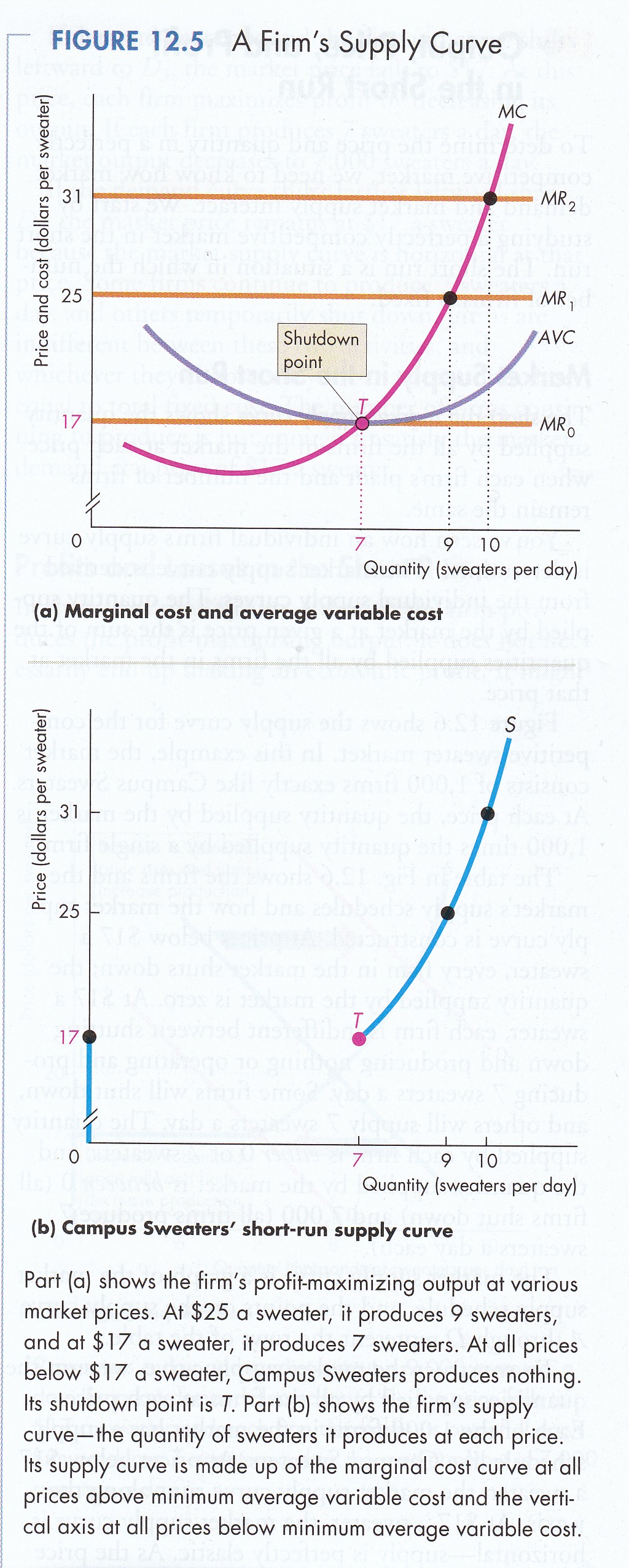
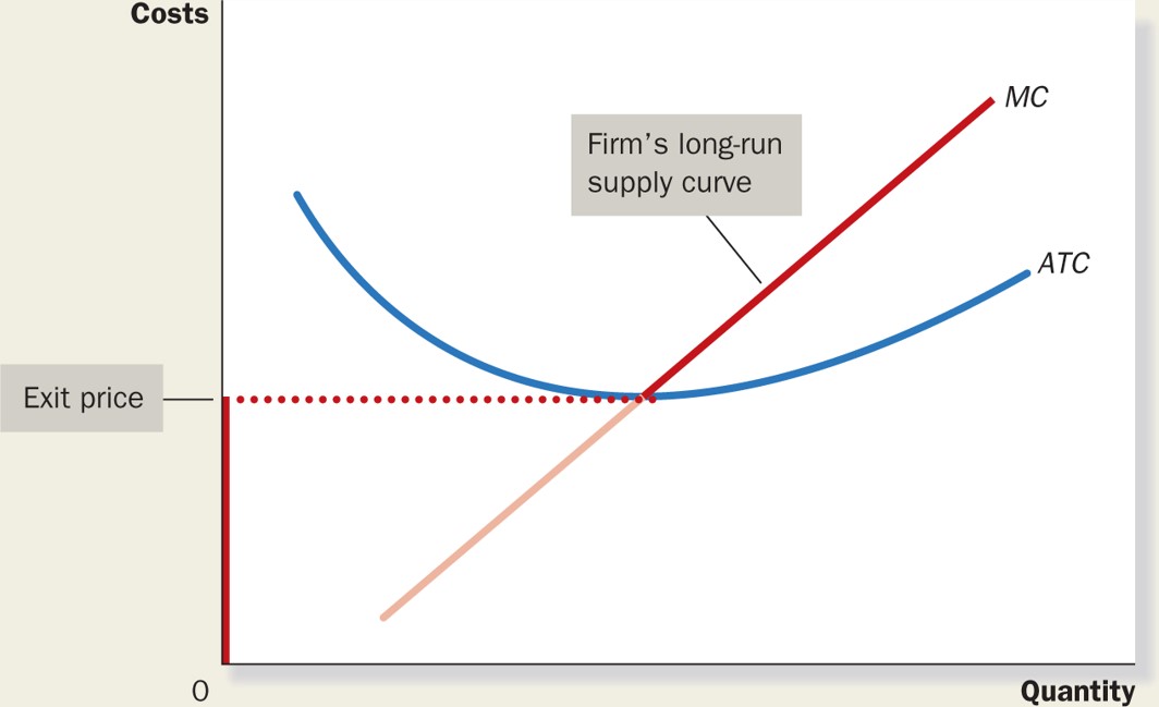
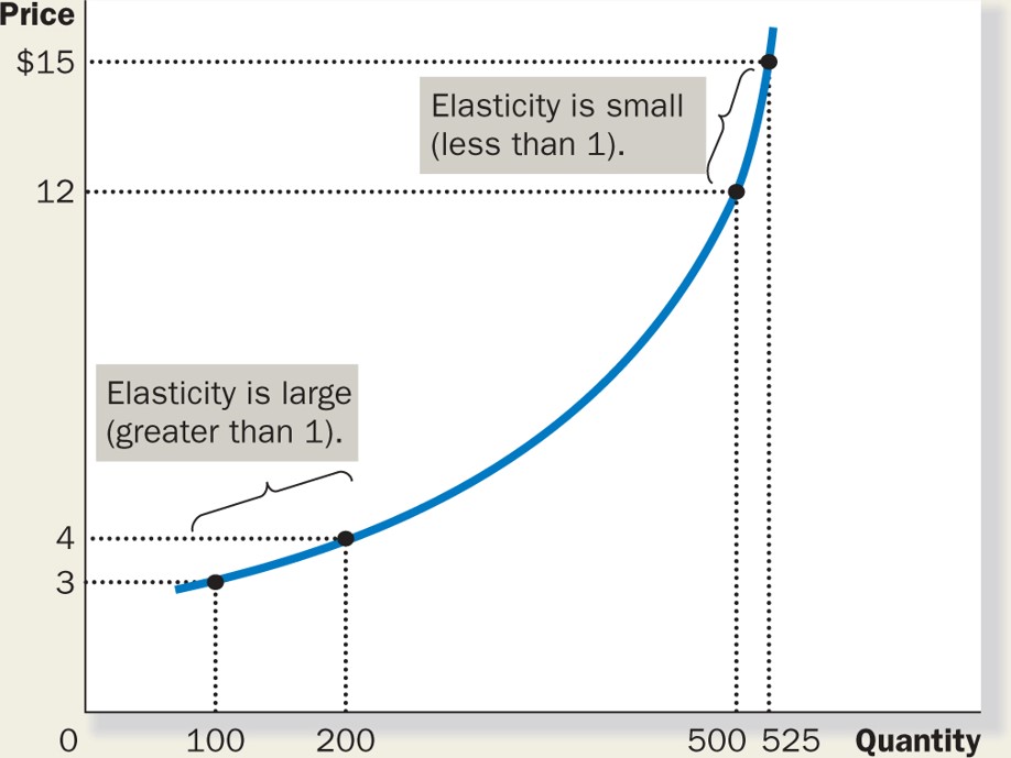
3. Supply Curve (MKM C14/295-307/ 277-88; 304-310; 283-288) The question remains: How much output will a firm be willing to supply given its cost constraints? Put another way: What is the firm's supply curve? This depends on how much the firm can get for its output, i.e. the price or revenue it receives per unit (P&B 7th Fig. 12.4, Fig. 12.5; R&L 9-4; CP TGQ #1, MKM Fig. 14.4). i - Shut Down (MKM C14/301-3; 284-5; 308-309; 286-287) If a firm cannot earn at least enough to cover all of its variable costs then in the short run it will shut down. This occurs at point B where marginal cost is equal to minimum average variable cost. This is called the 'shut down point'. If a firm earns a price higher than B it can cover all of its variable costs and some of its fixed costs and it will stay in business. Put another way, the firm will maximize profits by minimizing losses. ii - Break-Even (MKM C14/301-3; 284-5; 308-309; 286-287) In the long run, however, a firm must cover all costs - fixed and variable - or it will go out of business (M&Y 10th Fig. 9.3). This occurs at point D where marginal cost is equal to minimum average total cost. This is called the break-even point. At this point all factors of production - including entrepreneurship - are fully paid their opportunity cost. If the firm receives a price higher than the break-even point then it will earn economic or excess profits. Thus the supply curve of a firm is the marginal cost curve above minimum AVC (shut down point) in the short-run and above minimum ATC (break-even point) in the long-run. It is important to appreciate that the price or revenue a firm receives applies to each and every unit of output it sells. Accordingly it will produce to the point at which the cost of the next unit of output (MC) equals the price or marginal revenue (MR) it receives for that last unit. In effect, a firm earns a profit on each previous unit (if the price or revenue is greater than minimum AVC or minimum ATC in the short- and long-run, respectively). A firm thus maximizes profits (or minimizing losses) by producing at the point where price or marginal revenue equals marginal cost of the last unit of output. (16) MR = MC From the resulting cost function we can determine the supply curve of the firm, (R&L 9-5, MKM Fig. 14.4) i.e., how much it is willing to produce at each price. The supply curve is the marginal cost curve of the firm above the shut-down point in the short-run. If the firm cannot earn enough to cover all its variable costs, it shuts down. The curve will in the short-run be upward sloping reflecting the Law of Supply: the higher the price, the greater the supply; the lower the price the smaller the supply. In the long-run, firms can adjust the size of their plants (R&L 9-11, MKM Fig. 13.6) creating a series of short-run average and marginal cost curves. The long-run average cost curve is made up of an envelope of the minimum points of the short-run average cost curves. In the case of increasing return to scale industries at some point the most efficient plant size is achieved where long-run average cost is lowest. At this point optimal scale is attained and the short-run marginal cost curve, in effect, becomes the long-run marginal cost curve. iv - Elasticity (MKM C5/108-17; 101-09; 108-117; 97-105) Elasticity refers to the sensitivity of one variable to a one percentage change in another. Price elasticity of supply refers to the percentage change in the quantity of a commodity supplied compared to a one percentage change in its price (P&B 7th Ed Fig.4.8; R&L 13th Ed Fig. 4-6, MKM Fig. 5.6). The amount supplied can increase: a) more than proportionately, i.e. elasticity is greater than one - at the extreme a horizontal supply curve is perfectly elastic - a small increase in price results in a large change in the quantity supplied; b) proportionately, i.e. elasticity is equal to one (unitary elasticity); or, c) less than proportionately. i.e. elasticity is less than one (inelastic) - at the extreme, a vertical supply curve is perfectly inelastic - any change in price results in no change in the amount of the commodity demanded or supplied. (8) Q = g (L, K) where L, K & Q are fixed in the very short-run, L & Q variable, K fixed in the short-run K, L & Q all variable in the long-run (11) C = PLL + PKK where L = labour K = capital PK = price of capital PL = price of labour (16) Profit Maximization MR = MC
|