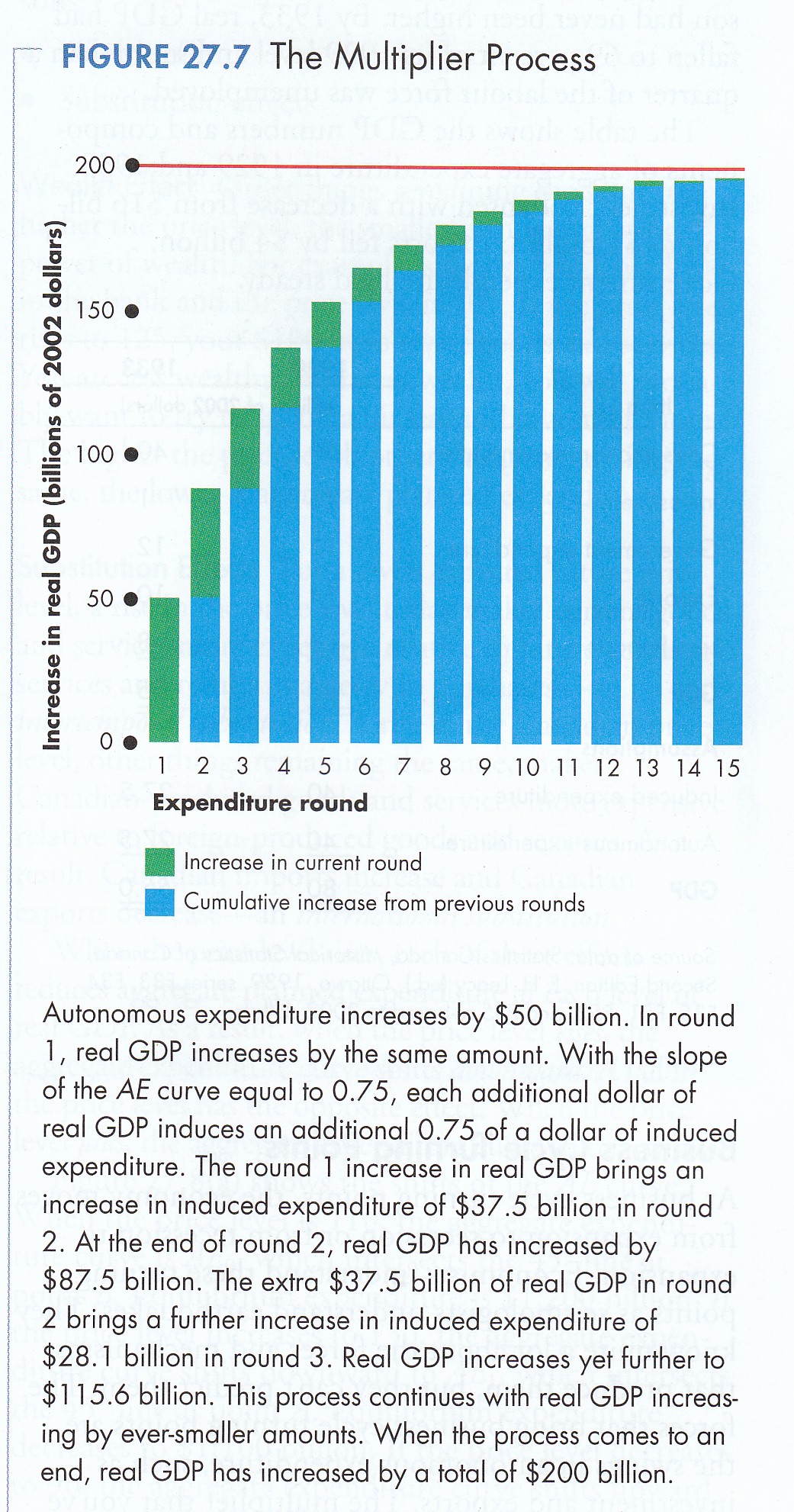
3. 4 The Multiplier (MKM C15/391-5; 366-370; C16/385-389; 362-365)

i -Concept

   Introduced by Keynes in his 1936 The General Theory of Employment, Interest and Money, the Multiplier shows by how many times an increase in any autonomous expenditure (I, G or X) increases Y.   In a way, the Multiplier is like throwing a pebble into a pond.  The initial ripple is followed by other ripples that stretch further and further out across the pond (P&B  7th Ed Fig. 27.5; R&L 13th Ed Fig. 21-9).   Thus if investment increases because firms anticipate lower interest rates or higher profits, they invest.  To invest they buy factors of production from households which therefore receive more income some of which they spend (1st ripple).  The goods and services purchased with this new household income are, in turn, made by firms that hire more factors of production to increase production that increases the income of other households some of which, in turn, is spent (2nd ripple).  And so on, and so on....

ii - Size

   We begin by assuming that the Aggregate Price Level is fixed in a closed economy and the Marginal Tax Rate (MTR) is zero.  Graphically (Figure 7), the size of the Multiplier depends on the slope of AE curve, i.e., the marginal propensity to consume or 'b'.  In a closed economy this is (1/1-b) where b = MPC and '1' represents total disposable income.  All things being equal, the steeper the slope of the AE curve, the larger the multiplier; the gentler the slope, the lower the multiplier (P&B 7th Ed Fig. 27.7).   Assuming b = .75 (75 cents of each additional dollar in income is spent on consumption) then (1/1-.75) = (1/.25) = 4.  It is important to note that the Multiplier is a process spreading out over time (P&B Fig. 25.8). 

iii - Consumption, Income Taxes & Imports

    The size of the multiplier depends on the slope of AE which, in turn, is determined by the marginal propensity to consume (MPC), the marginal tax rate (MTR) and, in an open economy, the marginal rate of imports (MPM).  All things being equal: the higher MPC, the steeper the slope of AE; the higher MTR, the gentler the slope; the higher MPM, the gentler the slope.

iv - Other Mutlipliers

In addition to the general Autonomous Expenditure Multiplier described above these include the:

a) Government Expenditure Multiplier;

b) Autonomous Tax Multiplier;

c) Balanced Budget Multiplier; and,

d) Impact of the Marginal Propensity to Import (MPM)

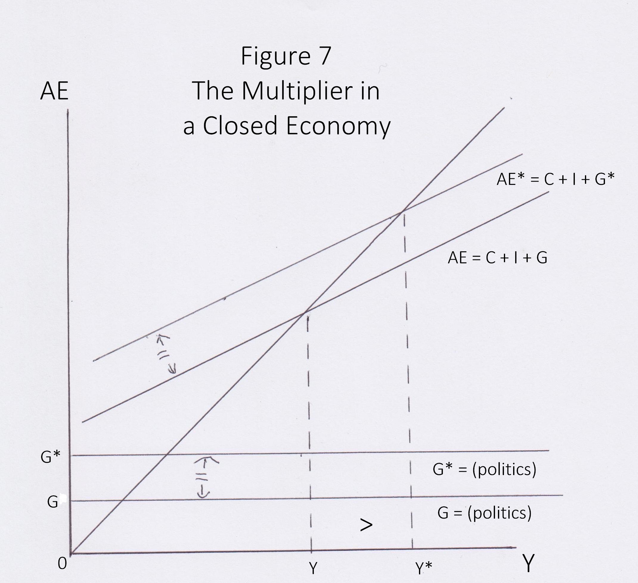
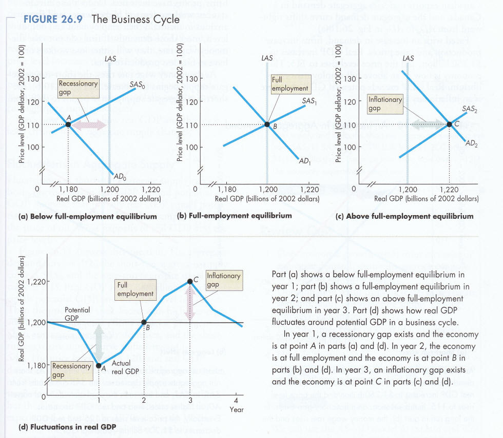
a) Government Expenditure Multiplier (GEM)
        The GEM is the same as the general Autonomous Expenditure Multiplier, i.e.,  GEM = 1/1-b = ∆Y/∆G.  For public policy this means an increase or a decrease in G has a multiplier effect on GDP - up or down.  Government, in other words, can use the Multiplier like a lever to increase or decrease GDP without doing it all itself.  Thus if G increases by $50 million with a Multiplier of 4 (as above) it causes GDP to increase by $200 million.  This is true assuming a fixed Aggregate Price Level, a closed economy and the Marginal Tax Rate (MTR) is zero.  As will be seen if P changes or we are in an open economy or the MTR is positive then the multiplier effect is reduced.

b) Autonomous Tax Multiplier (ATM)

There are essentially two kinds of taxes - induced and autonomous.  Induced taxes rise and fall as Y varies.  In this way induced taxes like income tax act as automatic stabilizers of the economy.  If Y goes up then the Marginal Tax Rate rises to a higher level (progressive taxation) and disposable income is reduced cooling the economy; if Y goes down the Marginal Tax Rate falls to a lower level and disposable income rises.

Autonomous taxes do not vary with real GDP but rather are determined by Government.  An increase in taxes decreases disposable income and hence consumption and therefore Y.  The decrease in Y will, however, be greater than the increase in taxes (P&B 4th Ed Fig. 26.9).  The Autonomous Tax Multiplier equals -b/1-b = ∆Y/∆T assuming a fixed Aggregate Price Level, a closed economy and the Marginal Tax Rate (MTR) is zero.  Thus if b = .75 then  ATM = .75/1-.75 = .75/.25 = 3.  Thus an increase in taxes of $50 million will lead to a decline in Y of $150 million.

The inverse of the ATM is the Multiplier associated with transfers. Transfers are like negative taxes, i.e., taxes are reduced. The Autonomous Transfer Multiplier is simply the negative of the ATM.  Another related concept  is 'tax expenditures' where Government selectively reduces taxes and losses revenue thereby.

iii - Balanced Budget Multiplier (BBM)
        The BBM is the amount by which a change in government expenditures is matched by a change in autonomous taxes.  The result is that the initial balance between government revenue and expenditure (deficit/surplus) is maintained.  The BBM requires that the effect of GEM (1/1-b) should exactly offset the effect of ATM (-b/1-b) so that ∆Y/∆G = ∆Y/∆T.  This is true assuming a fixed Aggregate Price Level, a closed economy and the Marginal Tax Rate (MTR) is zero.

iv - Impact of Marginal Propensity to Imports (MPM)

If, in a closed economy, we assume a MPC of .75, i.e., 75 cents of every dollar is spent on consumption then GEM is 1/1-.75 = 1/.25 = 4.  If, however, the economy is open and MPM is .1, i.e., 10 cents on every dollar is spent on imported goods then, AEM is 1/1-.75-.1 = 1/.65 = 2.86.  This again assumes a fixed Aggregate Price Level and the Marginal Tax Rate (MTR) is zero

iv - Business Cycle

    Economist study the business cycles - the ups and downs of the economy.  As will be seen the Multiplier plays a significant role in Government's management of the cycle.  According to the Dictionary of Economics and Business (Erwin Esser Nemmers, Littlefield, Adams, Totowa, New Jersey, 3^rd Ed., 1976, pp. 54-5), the business cycle is:

3.5 Aggregate Demand (MKM C14/340-7; 316-324; 328-333; 305-310)

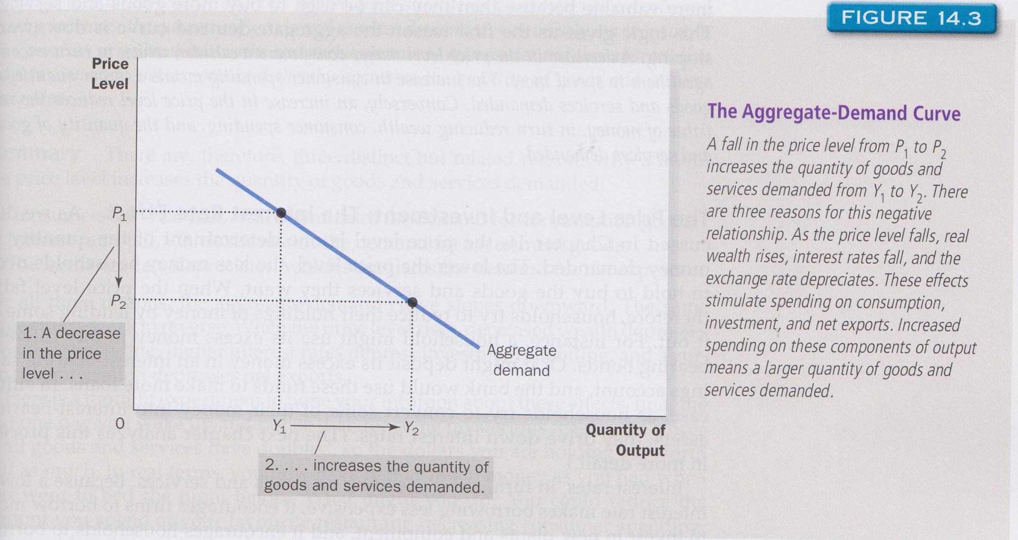
Aggregate Expenditure is calculated assuming a fixed Aggregate Price Level (P)   At a given P the various economic actors - households, firms, governments, exporters and importers - make their expenditure decisions: Y = C + I + G + X – M.  Change P and there is a different result.  For each level of P a different level of Y exists.  Plotting all different levels of P (graph below) with corresponding levels of Y and we can plot the Aggregate Demand Curve (ADC). The implications of changes in P for the multiplier effect will be explored later.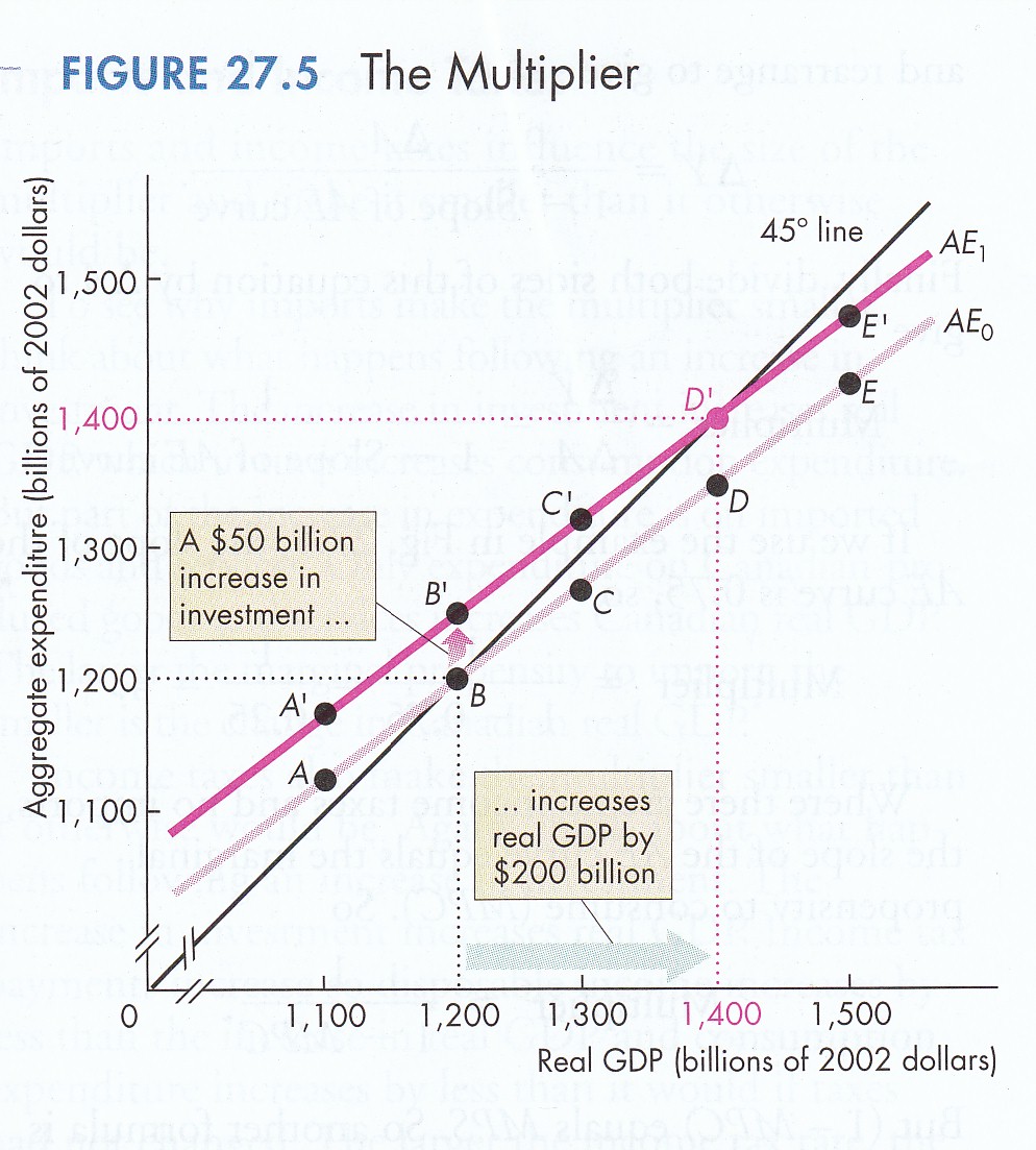