|
MACROECONOMICS + 3.0 Model 3.2 The Keynesian Model (cont'd)
(g) Aggregate Supply & Demand iii) Labour Demand & Supply Equilibrium
v) Increase in Money Supply & |
|
g) Aggregate Supply and Demand Analysis of Keynesian aggregate expenditure and the IS/LM curve has assumed that prices and wages are fixed. In effect the aggregate supply curve would, under these conditions, be perfectly flat (Fig. 8.1). Such conditions roughly correspond to a situation when the actual output of the economy is significantly below its capacity. Thus any increase in output need not affect wages or prices, i.e., increased output does not result in any inflationary pressure, e.g. during the Great Depression in which Keynes wrote the General Theory. Under normal conditions, however, an increase in output would tend to raise wages and prices resulting in the traditional upward sloping supply curve with increased output associated with rising prices.
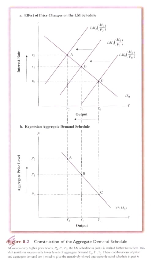
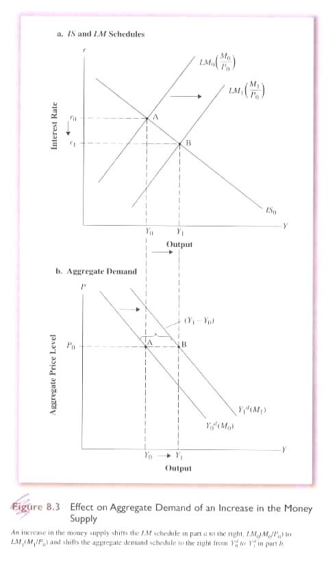
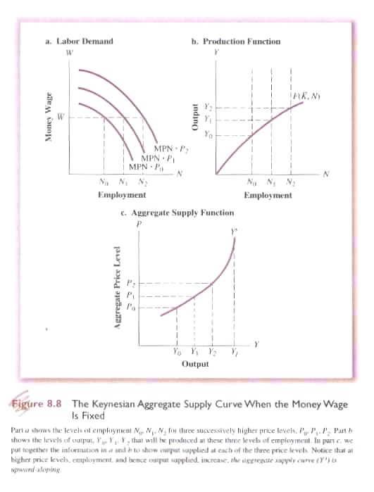
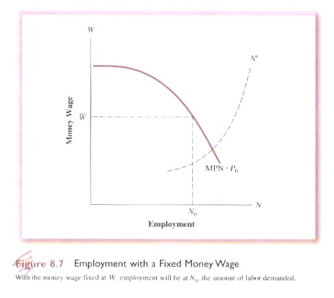
But how do price changes affect aggregate demand in the Keynesian model? First we can see how aggregate demand is determined through the interaction of the IS/LM curves (Fig. 8.2). But do price changes (ΔP) affect either of these curves. Equilibrium conditions for the IS curve occur when: (8.1) I(r) + G = S(Y) + T We know that G and T are determined autonomously by government and are assumed fixed in real terms, i.e., their real levels is unaffected by ΔP. Furthermore, it is assumed that I is determined by the ‘real’ interest rate. While ΔP may indirectly affect r, there is no direct effect on real investment. Similarly, real savings (S) is assumed to depend on real Y and will not be directly affect by ΔP. Thus with respect to the IS curve, ΔP will have no effect (Fig. 8.2). Equilibrium conditions for the LM curve occur when: (8.2) M/P = L(Y, r) Thus the real money supply equals the demand for money, i.e. demand for real money balances. M, however, represents the fixed autonomously determine nominal quantity of money provided by the monetary authorities. Given that households want to hold an appropriate real money balance ΔP will affect the real money supply and equilibrium in the money market (Fig 8.2a). Assuming that the nominal money supply is fixed at M0 and that P2 > P1 > P0 then as the price level rises the LM curves shifts to the left. From Fig. 8.2a we can calculate the varying level of Y given ΔP and from this information calculate the aggregate demand curve (ADC - Fig. 8.2b) that specifies the level of output at each price level. It is important to note that P refers to the ‘aggregate price level’, not to individual prices for goods and services. Thus ADC is affected by monetary factors through the LM curve as well as changes in real factors through the IS curve, e.g., real G, T, I and S. Factors that increase the level of equilibrium Y in the IS/LM model will cause the aggregate demand curve to shift to the right; factors that reduce equilibrium Y will cause the ADC to shift to the left. Consider an increase in the money supply from M0 to M1 (Fig. 8.3a). The increase shifts the LM curve to the right, i.e. from equilibrium A to B. Interest rates drop and Y increases from Y0 to Y1. Assuming the increase in M and Y are balanced there will not be a change in P. The result will be a shift in the ADC (Fig. 8.3b) and an increase in Y from Y0 to Y1 with no change in P. It should be noted that given these assumptions the shift in ADC at the same price level will result in an increase in Y that exactly matches the shift in IS/LM equilibrium, i.e., there is no multiplier effect. iii) Combining the Keynesian ADC with Classical Aggregate Supply If price and wages are not fixed then the impact of any policy change will depend on assumptions made about aggregate supply. Consider the case of an increase in G (Fig. 8.4). The ADC will shift to the right from Yd0 to Yd1. If the aggregate supply curve (ASC) corresponds to the Classical Model it is perfectly inelastic to ΔP (Ys0). The impact of ΔG will be an increase in prices with no effect on Y. If the aggregate supply curve (ASC) is upward sloping (Ys1 - normal economic conditions) then ΔG will result in an increase in Y but less than ΔG (Y0 to Y1) as some of the impact is absorbed in increased prices. If prices and wages are fixed then ASC will be horizontal (Ys2 – depression conditions) and ΔG will result in an equivalent increase in Y (Y0 to Y2). There will be, by definition, no ΔP. The aggregate supply curve in the Keynesian Model is, as in the Classical Model, based on the assumption of fixed capital and technology and variable labour reflected in a production function (see Fig. 8.8b). Given the production function a firm hire labour up to the point that the real wage is equal to the marginal product of labour (W/P = MPN), or, (8.1) W = MPN x P, i.e., the money wage equals the money value of MPN Through the horizontal addition of the labour demand curve for each firm, at each real wage rate, an economy-wide labour demand curve is derived. The labour supply curve in the Keynesian Model is not based on the assumption that labour faces a trade-off between leisure and the real wage, as in the Classical Model. Rather the supply of labour is based on the money wage in the presence of imperfect information about the price level. iii) Labour Demand and Supply Equilibrium In the Classical Model labour demand and supply equilibrium are assured by the assumption that money wages and prices are perfectly flexible. It is with this assumption that Keynes took exception. He believed that the money wage was not perfectly flexible and in fact subject to at least three forms of rigidity resulting from the nature of wage bargaining between unions and firms. First, wage bargaining tends to focus not just on the wage rate but also on the wage differential between different classes of workers, i.e., there is no an homogenous unit of labour but rather different forms and types. A given group of workers resist wage cuts not just because of the financial but also the status implications relative to other workers. A case in point is the wage differential between police officers and fire fighters. Over time a wage differential develops reflecting the relative worth of each group. Any attempt to alter that balance tends to be resisted. Second, unions negotiate contracts for specific time periods, e.g., two or three years. During that period the money wage cannot be changed by firms. Third, even when there is no formal contract between unions and firms there is a tendency – a convention - to maintain the money wage for a given time period. Taken together these three factors tend to make the money wage ‘sticky’ rather than perfectly flexible as assumed in the Classical Model. At the extreme such ‘stickiness’ becomes a fixed money wage and equilibrium is not established (Fig. 8.7). Given a fixed money wage, the actual level of employment is determined purely by the demand for labour. This means that the money wage does not adjust to ensure full employment. Rather there can be a disequilibrium in which the amount of labour demanded at the fixed money wage is less than what labour is willing to supply. If money wage rates are fixed (or sticky) but prices are flexible then firms will vary the amount of labour they employ based on the price they receive for their output always ensuring that W/P = MPN. Thus if price goes up (and the money wage remains fixed) companies will employ more workers (Fig. 8.8a). Thus at different levels of P output will change and the supply curve for the firm can be calculated. Taking price information from Fig 8.8a and output information from Fig. 8.8b the supply curve for a firm can be calculated as shown in Fig. 8.8c. The horizontal summation of the supply curve for each firm at each price level generates the aggregate supply curve for the economy. The result, unlike the vertical aggregate supply curve of the Classical Model, is an upward sloping supply curve showing that as price increases output increases.
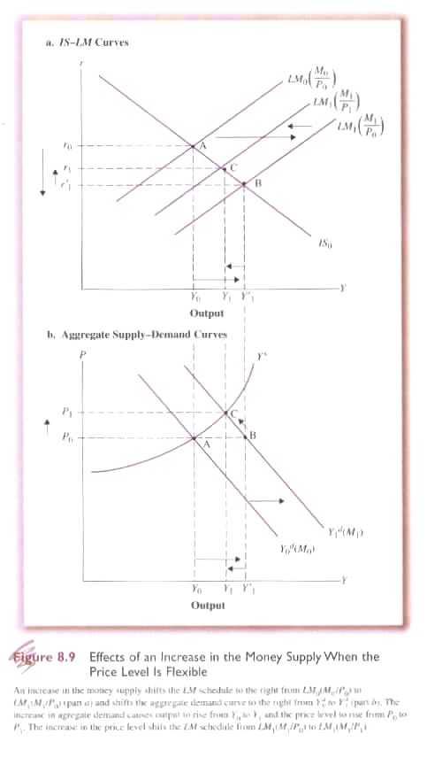
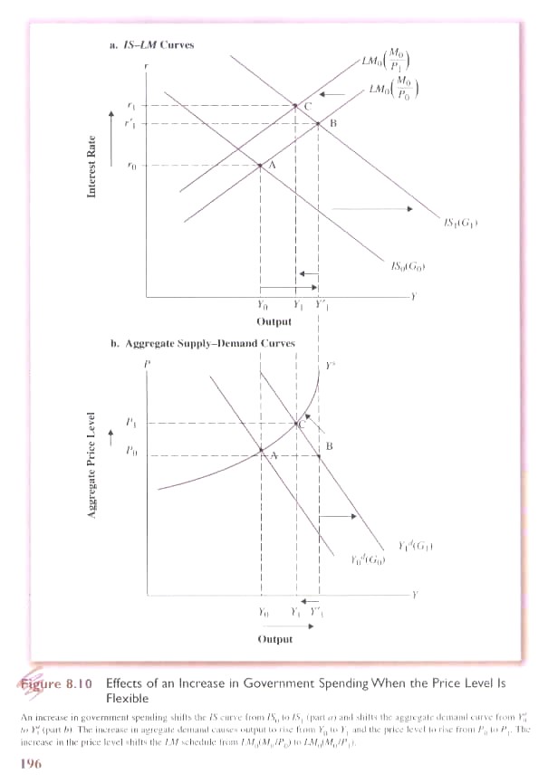
v) Impact of Changes in the Money Supply and Government Spending As we have seen an increase in the money supply will shift the LM curve from equilibrium at A downward to the right at equilibrium point B (Fig. 8.9). If prices are fixed the result will an increase of output from Y0 to Y’1. But if output increases (movement along the aggregate supply curve), the price level will rise. The effect of a price increase is to reduce the real money supply shifting the LM curve back from equilibrium at B upwards to C. In turn output will fall back from Y’1 to Y1. An increase in government spending has a similar effect (Fig. 8.10). An increase in G shifts the IS curve up to the right from equilibrium at A to B. If prices are fixed output increases from Y0 to Y’1. If prices are flexible, however, the increase in output is accompanied by an increase in prices that effectively reduces the real money supply shifting the LM curve up to the left from equilibrium at B to a new equilibrium at C. In turn output will fall back from Y’1 to Y1.
vi) Classical v. Keynesian Theories of Labour The Classical Model assumed that labour, in making a trade-off between work and leisure, based its decision on the real wage. Accordingly, an increase in the real wage led to an increase in the supply of labour. The Keynesian Model, on the other hand, assumes that labour makes its decision between work and leisure based on the money wage. It is here that Keynes introduced the idea of ‘imperfect knowledge’. Thus while labour would obvious know, through bargaining, the money wage it has no way of knowing the actual aggregate price level. Rather labour depends on an expectation of the aggregate price level based on past experience. The Keynesian labour supply function is: (8.5) Ns = t(W/Pe) where W is the money wage and Pe is the expected price level. In effect, this amounts to the labour supply depending on the real wage but the real wage defined as money wage divided by the expected price level. As suggested above, in general labour makes its expectation of the price level based on past experience, or (8.6) Pe = a1P-1 + a2P-2 + a3P-3… anP-n where P-i refers to successively more distant past periods and ai refers to the weight attached to each of those periods. This assumes that accurate information about past price levels can be obtained at a ‘reasonable’ cost and thereby be expressed simply as in Eq. 8.6. It also assumes a backward-looking behaviour. Furthermore, Keynes assumed that adjustment in expectations would change only slowly to past price behaviour. Thus expectations do not change immediately in response to current economic conditions but only slowly as present conditions slide into the past.
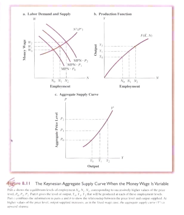
Labour supply and demand thus varies with the money wage assuming a relatively fixed expectation of the aggregate price levels (Fig. 8.11a). Firms, however, actually demand labour based on the real wage which is a function of the marginal productivity of labour (MPN), the money wage and the price level. It is assumed that firms do have a good idea of at what price level they can sell their output. Accordingly the labour demand curve will tend to shift to the right as the price level increases. The labour supply curve, however, is based on the relatively fixed (in the short-run) expected price level. As the price level increases firms increase output but to do so they must hire more labour. They can do so, however, only by increasing the money wage. As employment rises, output increases (Fig. 8.11b). Taking information from Fig’s 8.11a and 8.11b the aggregate supply curve can be calculated (Fig. 8.11c). As is apparent, given the assumptions, even if money wages are flexible the aggregate supply curve is upward sloping not vertical as in the Classical Model.
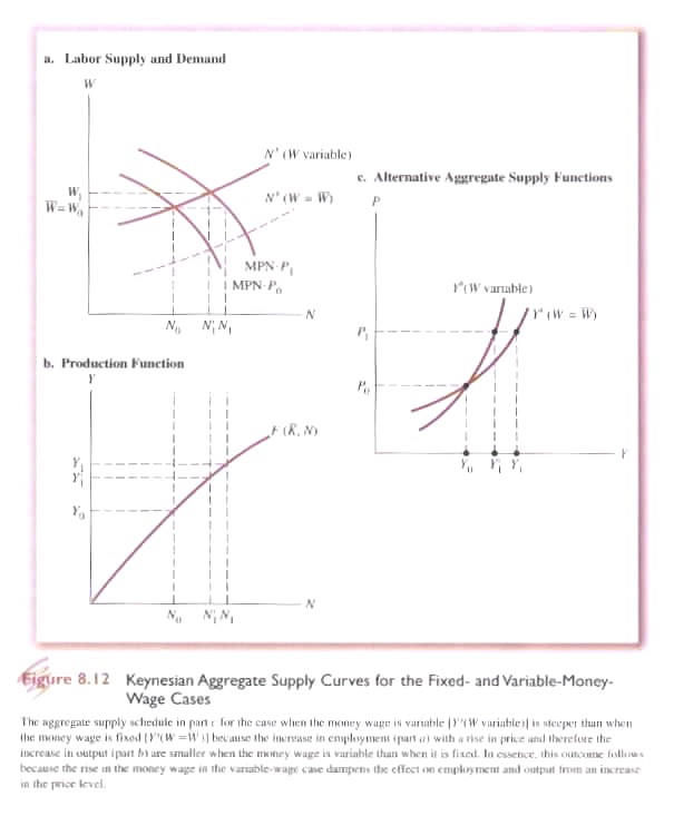
viii) Policy Effects of a Variable Money Wage Given an upward sloping aggregate supply curve a shift in aggregate demand will have an effect on output (unlike the vertical ASC in the Classical Model where any change of demand is converted entirely into price increases). However, if we compare the situation in which money prices are fixed with when they are variable the ASC is more inelastic in that later case (Fig. 8.12). Why? If the money wage is fixed then any increase in prices elicits an increase in output from Y0 to Y1 (Fig. 8.12c). The fixed money wage corresponds to a surplus of labour, e.g. during a depression or recession. The only factor affecting the increase in output is the decline in MPN due to diminishing marginal returns that limits the increase in employment. If the money wage is variable (corresponding to full employment at the existing money wage) then a price increase elicits an increase in output that in turn requires more labour that in turn requires a higher money wage. This means that the labour cost of firms increase as output rises. The higher money wage constrains the amount of additional labour employed for a given price increase. In effect, the ASC with a variable money wage is steeper and more inelastic than when the money wage is fixed and the increase in output Y’1 is accordingly less than Y1 (Fig. 8.12c). In the Classical Model the vertical ASC reflects the assumption that output is purely supply-determined. Changes in the ADC are translated not into increased output but only price increases that are exactly matched by rises in the money wage. Accordingly any change in policy such as an increase in government spending or the money supply can have no effect on output and employment. By contrast in the simple Keynesian Model with fixed money wages and prices changes in policy cause the ADC to shift (either through the IS curve in the case of government spending or the LM curve in terms of changes in the money supply). The impact of policy changes work their way through with the full impact of policy multipliers, i.e., nothing is lost to price increases. The implicit assumption is that the ASC is horizontal and offers no impediment to policy changes (Fig’s 8.1 & 8.4). This situation corresponds to a state of economic depression where there are so many unemployed resources that increased output does not result in increases in prices or the money wage. In the Keynesian Model with fixed money wages but flexible prices which more closely approximates normal economic circumstances an increase in output is limited by the diminishing marginal product of labour, i.e. with fixed capital and technology the addition of more units of labour eventually results in a smaller and smaller increase in output per additional unit of labour. Thus firms hire only to the point where the real wage is equal to MPN will increase employment only if price increases, i.e. profits rise. The result is an upward sloping ASC reflecting the fact that firms will increase employment and output only if price increases. In the Keynesian Model with both variable prices and money wage, firms will similarly increase output only if price increases. However the response of firms to price increases is tempered not only by diminishing MPN but also the fact that the money wage must be increased if additional labour is to make itself available. Accordingly the, ASC is upward sloping as in the previous case but steeper reflecting the fact that a given price increase will have a smaller impact on output than when the money wage is fixed.
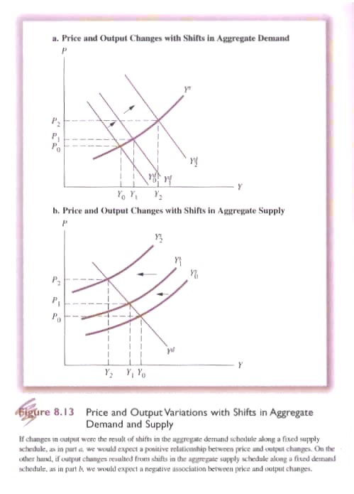
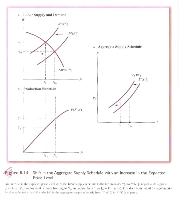
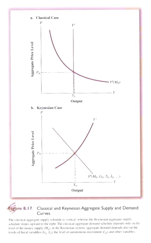
(h) Shifts in the Aggregate Supply Curve So far we have considered shifts in the aggregate demand curve caused by policy variables like increased government spending (G), taxes (T) or the money supply (M). The effects of changes in the ADC are clear: an increase in G or M will shift the ADC to the right and given an upward sloping ASC prices and output will rise. A decrease in G or M will have the opposite effect shifting the ADC to the left. In the case of ΔT, the movement is in the opposite direction (Fig. 8.13a). But what can cause the ASC to shift (Fig 8.13b)? In effect we have assumed that demand factors are variable (C, I, G, T, X, Z) while supply factors, with the exception of labour, are fixed (capital, raw materials and technology). And even labour has been constrained to changes in the money wage with Pe considered relatively fixed. If, however, we change Pe the ASC will shift (Fig. 8.14). In fact as experience accumulates expectations on the part of labour concerning prices will change and shift the ASC. Similarly, any change in capital, raw materials or technology will similarly cause a shift in the ASC. If the quantity of capital increases the production function will shift; if the price of raw materials, e.g. oil, increases the production function will shift, and, of course, if technology changes the production function will change. Any of these changes in supply factors will cause the ASC to shift. The impact of such a shift will depend on the shape of the ADC. Thus if the ADC is very elastic a shift in the ASC will have a strong effect on prices and output. If the ADC is relatively inelastic the shift of the ASC will have a smaller effect. In both the Classical and Keynesian Models it is the interaction of the ASC and ADC that determine prices and output of an economy. In the case of demand we have seen that the Classical Model did not have an explicit theory of demand. An implicit theory was, however, developed using the quantity theory of money. (8.8) MV = PY where M is the money supply fixed by the monetary authority, V is the velocity or turn over of money which was assumed to be an institutionally established constant, P is the price level and Y is the output of the economy. Alternatively, in the Cambridge formulation (8.9) M = Md = kPY where k was a constant representing the amount of cash households held. In the Classical Model an increase in M would result in demand increasing but translated into price increases because the ASC was assumed to be determined purely by supply factors (Fig. 8.7a). The primary adjustment or stabilizing mechanism was the interest rate or the cost of money. Thus if G increased, and was financed by borrowing, interest rates would rise driving down I to accommodate government borrowing. In effect only monetary or nominal factors would shift the ADC and such shifts would be absorbed through price changes with no change in output or employment. By contrast the Keynesian ADC would shift in response to changes in demand factors such as C, I, G, X or Z. Furthermore, Keynes believed that instability of I, in response to changing business expectations, would cause shifts in the ADC and contribute to instability in prices and output. With respect to the ASC, the Classical Model assumed it was perfectly inelastic and determined strictly by supply factors. Labour responded to changes in real wages so that increases in prices would be matched by increases in the money wage to maintain the real wage. Prices and money wages were assumed to be perfectly flexible. In the Keynesian Model it was assumed that labour responded to money wages together with relatively stable expectations concerning prices (Pe). Furthermore, Keynes assumed that the money wage tended to be ‘sticky’ rather than flexible which meant that if prices rose the money wage did not. This meant that a price increase would lead to higher profits for firms and higher output leading to an upward sloping ‘short-run’ ASC (Fig. 8.17b). The stickiness of money wages meant that there was no automatic adjustment to return the economy to full employment. Keynes did not deny that an adjustment would in the long-run take place but said “In the long run we are all dead”. These differences of opinion concerning the ASC and ADC result in dramatically different policy implications that will be examined later in this course.
|