MACROECONOMICS +
3.0 Model
3.2 The Keynesian Model (cont'd)
We have seen that when money and the cost of money (the interest rate) were introduced to the Classical Model there was no ‘real’ effect. Prices increased or decreased (including the price of money) but ‘real’ output did not change. In fact, the aggregate supply curve was vertical (perfectly inelastic). ‘Real’ demand (as opposed to the demand for money) was in effect given by Say’s Law: supply creates its own demand. But what happens in the Keynesian Model?
To begin it is assumed, as in the Classical Model, that the supply of money (M1) is, in effect, fixed by the monetary authorities. The demand for money in the Keynesian Model, however, is not the same. Assuming income can be held either as money, spent or converted into interest earning assets (bonds), for Keynes there were three main reasons for holding money as cash:
i) transaction demand
ii) precautionary demand;
iii) speculative demand; and,
iv) total demand.
i) Transactional Demand
Money would be held as a medium of exchange for use in transactions, i.e. to pay bills. Transactional demand would vary positively with the volume of transactions (TD) and income was assumed to be a good measure of TD. Further there would be pressure to ‘economize’ on one’s transactional cash balance. That pressure emanated from the rate of interest. While there are brokerage and other fees associated with buying bonds (making small purchases less attractive, i.e. the ‘real’ rate of return being r – f where f stands for fees), the higher the interest rate the higher the final rate of return and so individuals and households are more likely to compress their transactional demand for money as the interest rate rises. In conclusion, TD varies positively with income and negatively with the rate of interest.
While Keynes did not stress the impact of r on TD businesses through their cash management practices do. Firms with a large volume of transactions will reduce their TD as r rises.
ii) Precautionary Demand
Individuals always have a demand for cash on hand to meet emergencies – medical or repairs. Accordingly some cash will always be held in cash and Keynes assumed the amount of precautionary demand (PD) would vary positively with income. To simplify our analysis it will be assumed that PD can be subsumed under TD as an ‘unexpected’ transaction demand for money.
iii) Speculative Demand
Speculative demand for money (SD) represented an original contribution to the theory of money by Keynes. He argued that given uncertainties about future interest rates and the relationship between interest rates and price of bonds (specifically capital loss or gain on their value) meant that there would be times when individuals would hold on to cash. If you buy a bond to day you are committing part of your income to something that will pay a given rate of interest say r1. The price of the bond is sometimes called its yield measured by the purchase price – say $1,000 and its coupon or interest rate is, say 5%. If tomorrow the interest increases to r2 – say 10% - you will, in effect, lose (r2 – r1). Furthermore, if you try and sell your old bond its price must be decreased to yield an effective rate of r2. The difference in what you paid for the bond and the price at which you must sell it to generate an effective yield of r2 is called a ‘capital loss’. For example, while the old bond cost you $1,000 and generates a 5% return, the bond could be sold tomorrow only for $500 if the buyer is to get the going rate of 10%.
Keynes argued that the uncertainty would lead some individuals to hold onto cash in order to earned a higher rate tomorrow and avoid capital losses. And vice versa, if interest rates were expected to fall then speculative demand for money would fall as higher yielding bonds are purchased today in the hope both of a lower interest rate tomorrow and the chance of ‘capital gains’. Thus a $1,000 bond yielding 10% will sell for $2,000 if the interest rate drops to 5% tomorrow.
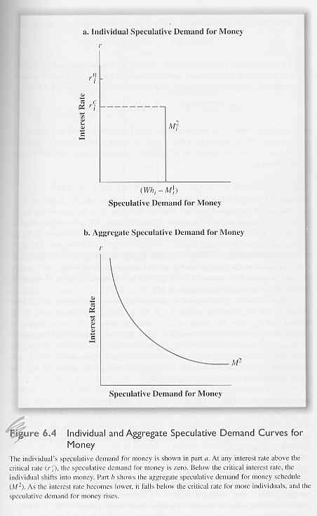
In effect, Keynes assumed that different individuals had different views about future change in the interest rate. Each had preconceptions of what was the ‘normal’ rate of interest. Those who thought ‘the normal rate’ was higher than today’s rate would tend to have a higher SD; those who thought the normal rate was less than today’s rate would have a lower SD. At ‘very’ lower current rates most individuals will have a high SD in anticipation that rates will rise tomorrow and to avoid capital losses. If enough individuals hold on to cash a ‘liquidity trap’ is reached. This is the point at which the demand for money (liquidity) is perfectly elastic with respect to the interest rate. This is reflected in 7th Ed Fig. 6.4b & 8th Ed Fig. 7.4b [n.b. please note that the following equations are numbered according to the 8th Ed.] where the curve tends to flatten out at the bottom. In liquidity trap any increase in the money supply yields no fall in the interest rate. Such a situation arises when the yield on income earning assets is so low that the risk of holding such assets is so high (capital losses if rates rise) that investors prefer to hold on to any increase in the money supply in liquid form.
iv) Total Demand
Total demand for money in the Keynesian Model or MD = TD + PD + SD where TD and PD vary positively with income and negatively with respect to interest rate while SD does not vary with income but negatively with respect to interest rates. Taken together we can say:
(7.3) Md = L(Y, r)
and if we assume the function is linear then
(7.4) Md = co + c1Y – c2r where c1 >0, c2 >0 and
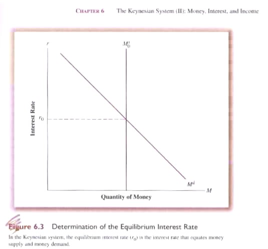
c0 is the minimum amount of cash that must be held; c1 is the increase in money demanded per unit increase in income and c2 is the decrease in money demanded per unit increase in the interest rate. Assuming linearity (that is a straight line) the total demand for money is downward sloping relative to the rate of interest (7th Ed Fig. 6.3; 8th Ed Fig. 7.3).
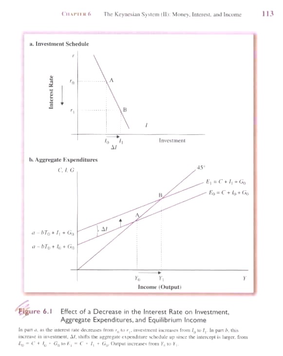
Firms borrow money from households to finance investment projects by issuing stocks and bonds or borrowing from financial institutions. The price they pay for this money is the interest rate. As previously noted Keynes assumed firms had an investment schedule that measured the expected profit rate to be earned from alternative projects mapped against the rate of interest. If the expected profit less the cost of money was positive, a firm ceterus paribus will undertake the project; if negative, then the project would not be undertaken.
If the interest rises, then business borrowing declines; if interest falls, borrowing increases (7th Ed Fig. 6.1; 8th Ed Fig. 7.1). If investment increases then aggregate expenditure shifts up by the autonomous increase in I. This increase through the aggregate expenditure multiplier will lead to an even larger increase in income. Accordingly, the interest sensitivity of aggregate demand is important in determining appropriate monetary polices.
3. Theory of the Interest Rate
In effect the interest rate is determined in two distinct markets. The first is the market for bonds. The second is the market for money itself. Put another way, one can hold one’s wealth (assets) as either money or bonds, i.e.,
(7.1) Wh = B + M
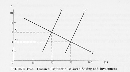
At a given rate of interest there will be a demand for money (Eq.’s 7.3 & 7.4) and a supply of money provided by the central bank (7th Ed Fig. 6.3; 8th Ed Fig. 7.3) and an equilibrium value for R that matches the demand and supply of money. Alternatively there is a demand for and a supply of bonds and an equilibrium value for r that balances supply and demand (Shapiro Fig. 17.6). In overall equilibrium the resulting interest rate will be the same.
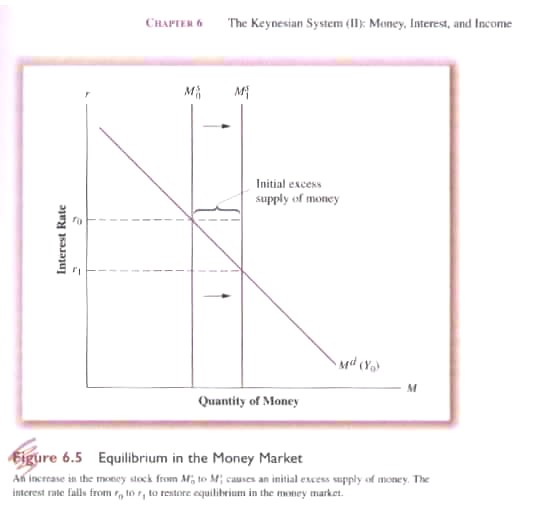
7th Ed Fig. 6.5 & 8th Ed Fig. 7.5 demonstrates initial equilibrium in the money market followed by an increase in the money supply. Unlike the Classical Model, the increase in the money supply not only lowers r it also results in an increase in I that leads to growth in income (7th Ed Fig. 6.1; 8th Ed Fig. 7.1).