MACROECONOMICS +
3.0 MODELS
3.1 The Classical Model
(b) Money, Prices & Interest
3.1.8 The Quantity Theory of Money
Having determined output and employment equilibrium in the Classical Model we turn to price determination which brings demand into play. In summary, the quantity of money determines aggregate demand that in turn determines the price level.
3.1.8 The Quantity Theory of Money
The starting point is the ‘equation of exchange’. At any given time there are a certain number (or volume) of transactions (i.e. T = the number of buy/sells) in the economy. T is financed with money that can, however in the same time period, be used over and over again (I buy and give you money in the form of dollar bills; you then use the same bills to buy something from some one else who in turn, and so on and so on). The rate at which the same bills ‘turnover’, that is the number of transactions financed with the same bills, is called the velocity of money (V). Of course each buy/sell has, in a given time period, an associated price (P) or, in the case of the overall economy, a price index for the huge range of goods and services bought and sold. Accordingly the actual quantity of money required to conduct all transactions in the economy is only a percentage of the monetary value of total output and purchases. This is summed up in the equation of exchange (EE) as:
Eq. 4.1 MV
![]() PTT or,
PTT or,
- the quantity of money times its velocity is identical to the price (level) times the volume of transactions.
This presentation of EE (Eq. 4.1) is an identity in that V is derived as a residual, i.e.,
Eq. 4.2 VT
![]()
Furthermore, in this version transactions include not only newly produced goods and services but also second-hand ones. Expressed with respect to only new goods and services that correspond to factor income then EE is:
Eq 4.3 MV
![]() PY where
PY where
- Y is the output of current good and services and P is their price index.
Again EE is an identity if V is calculated as a residual, i.e.,
Eq. 4.4 V
![]()
It will be this version of EE with which we will work in the Classical Model. On its own, however, EE does not explain its component parts. A number of economists including Irving Fisher attempted to explain the value of its component variables, with the exception of the P, based on exogenous factors. First, as we have seen, Y (real output) is determined in the Classical Model by supply factors (e.g. K, MPN, N, W/P, technology and population). Furthermore, money is considered simply a medium of exchange and its quantity is, implicitly to this point, exogenously determined by monetary authorities, i.e. the central bank.
V is considered also to be determined exogenously by payment habits (weekly, bi-weekly, monthly) and payment technology, e.g. cheques, point of sales, credit and debit cards. Thus the shorter the payment period, the less cash will tend to be held at anyone time increasing the velocity of money. Similarly chequing and credit purchasing tend to increase velocity, i.e. a fewer number of bills finances transactions. In short, velocity is determined by institutional factors that can be considered fixed in the short run.. If V is determined exogenously rather than as a residual then EE ceases to be an identity. With Y fixed in the short run by supply-factors and V being fixed in the short run by institutional factors, EE becomes:
Eq. 4.5
![]() or
or
Eq. 4.6
![]()
An alternative interpretation was offered by the Cambridge School known as the Cambridge approach or the Cambridge cash-balance approach. This approach stressed that people held money (cash balance) for its convenience, compared to other stores of value, in conducting transactions. However holding cash means that no interest will be earned from investing in productive activities. Accordingly, how much cash would people hold? In essence the demand for money was a function of their income, i.e.,
Eq. 4.7 Md = kPY where
- Md = the demand for money;
- k = a proportion of nominal income;
- P = the price level; and,
- Y = real income.
Given, according to the Cambridge approach, that cash was desired due to its usefulness in transactions and that the volume of transactions was a function of income then the demand for money varies according to level of income.
In equilibrium, the supply of money (exogenously determined by monetary authorities) would equal the demand for money, or,
Eq. 4.8 Ms = Md
= kP![]() where,
where,
- k is assumed fixed in the short run; and,
- Y is determined, as before, by supply factors.
The Fisher version (Eq 4.5) and the Cambridge approach (Eq. 4.7) become roughly the same if V = 1/k. Thus if people hold 1/4th of their nominal income as cash then the number of times the average dollar is used equals four.
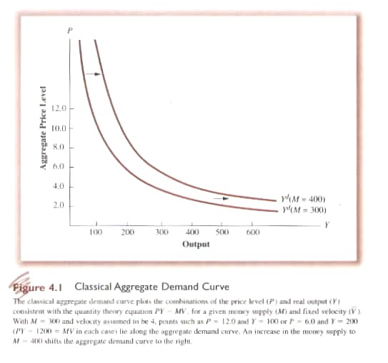
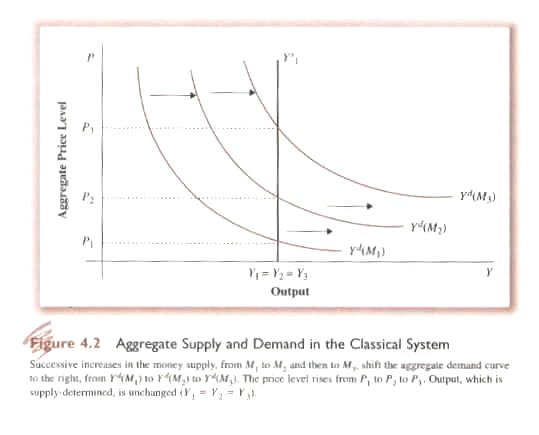
The big change with the Cambridge approach is the formal introduction of the demand for money. It also allows an assessment of the impact of the quantity of money on the price level (Fig. 4.1). If the quantity of money increases but output is fixed then people will use the extra cash to consume or invest. Increased demand for goods raises their prices: too much money chasing too few goods. If Y is fixed (Fig. 4.2) as assumed in the Classical model and k is constant then a new equilibrium will be established at which the increase in money leads to a proportionate increase in price – same output, higher prices, i.e. inflation.
3.1.10 Classical Aggregate Demand Curve
The quantity theory is in fact an implicit theory of aggregate demand in the Classical Model (Fig. 4.2). Given that supply is fixed then at any given quantity of money (M1) there will be a corresponding demand that varies inversely to the price level, i.e. a downward sloping demand curve and there will be an equilibrium price level that ‘clears the market’, i.e. demand equals supply. If the quantity of money is increased (M2) the demand curve will shift to the right, i.e. at the same price level demand will increase but, again, supply is fixed. A new equilibrium will be established at the same level of output but at a higher price level.
3.1.11 The Classical Theory of the Interest Rate
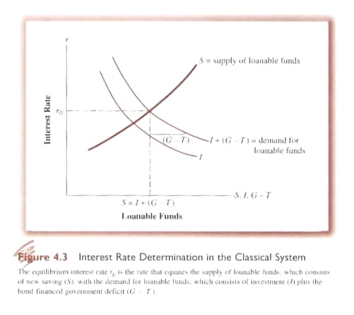
In the Classical theory, using the Cambridge approach, the interest rate (the price of money) measures the cost of holding cash. At a given level of k, individuals therefore have what is called ‘loanable funds’ (hence Keynes’ called the Classical Model of interest the ‘Loanable Funds Theory’. Beyond their need for money for transactional purposes, cash can serve as a store of value but yields no return so individuals will tend to hold their excess money in interest yielding securities. The Classical Model assumed that the rational individual would not hold excess money in the form of cash.
Firms borrow funds from individuals in order to build new plant and equipment that eventually will increase Y. However, any investment is associated with a corresponding rate of return. A firm can only earn a profit on a given investment if its rate of return is greater than the opportunity cost of money, i.e. the interest rate. In the Keynsian Model the alternative investment opportunities formed a Marginal Efficiency of Investment Schedule with alternative projects ranked according to their estimated rates of return. Projects with rates above the interest rate would be undertaken while those with rates below the current interest rate would not (Fig. 4.3).
D
emand for loanable funds varies inversely with the interest rate. Similarly there is a supply of loanable funds that varies directly with the interest rate, i.e. an upward sloping supply curve. Equilibrium is reached when the two curves cross. An exogenous change in demand conditions is illustrated in Fig. 4.4. If demand shifts to the left initially there is a greater supply of loanable funds than demand. This causes the interest rate to fall until a new equilibrium is established.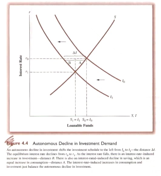
The interest rate played a critical role in the Classical Model in ensuring full employment. Output is fixed and based on supply factors especially the self-adjusting labour market. The decrease in the interest rate in Fig. 4.4 causes consumption to go up exactly balancing the fall in investment and maintaining aggregate private demand (C + I).